
Solving Open-Pit Long-Term Production Planning Problems with
Constraint Programming
A Performance Evaluation
Ricardo Soto
1,2
, Broderick Crawford
1,3
, Boris Almonacid
1
, Franklin Johnson
1,4
and Eduardo Olguín
5
1
Pontificia Universidad Católica de Valparaíso, Av. Brasil 2950, Valparaíso, Chile
2
Universidad Autónoma de Chile, Av. Pedro de Valdivia 641, Santiago, Chile
3
Universidad Finis Terrae, Av. Pedro de Valdivia 1509, Santiago, Chile
4
Universidad de Playa Ancha, Av. González de Hontaneda 855, Valparaíso, Chile
5
Universidad San Sebastián, Bellavista 7 Recoleta, Santiago, Chile
Keywords: Intelligent Problem Solving, Decision Support Systems, Optimization.
Abstract: Open pit mining problems aims at correctly identifying the set of blocks to be mined in order to maximize
the net present value of the extracted ore. Different constraints can be involved and may vary the difficulty
of the problem. In particular, the Open-Pit Long-Term Production Planning Problem is one of the variants
that better models the real mining operation. It considers, among others, limited processing plant and mining
capacity as well as slope and grade blending constraints. During the last thirty years, different techniques
have been proposed to solve the multiple variants of the open pit mining problem; however, the resolution
via constraint programming has not been reported yet. In this paper, we present a performance evaluation of
seven constraint programming solvers for the open pit mining long-term scheduling problem. We illustrate
interesting and comparative results on a set of varied open pit mining instances.
1 INTRODUCTION
Open pit mining refers to a method of mineral
extraction in which the ore body is reached by
opening a large ground surface along a mine. The
orebody is commonly discretized to be regarded as a
three-dimensional array of blocks, where each block
has different attributes, e.g., tonnage, extraction cost,
estimated ore content, and expected in-ground value.
A main aim of mine planning is to correctly select
the blocks to be mined in order to maximize the total
profit from the process. Different constraints can be
involved and may vary the difficulty of the problem
such as, a limited processing plant capacity, the need
for a balanced mining flow during a given time
horizon, the satisfaction of a given metal demand, or
simply to handle the extraction of several
predecessors blocks to reach a valuable one. The
study of open pit mining problems dates back to the
1960s, and different variants have been reported.
The simplest one is the ultimate pit problem (UPIT)
[Ahuja et al., 1993) also known as maximum-weight
closure problem. This problem aims at finding the
set of profitable blocks within the ore body that
maximizes the net present value (NPV). The only
constraint involved is about precedence among
blocks for extraction, also known as slope
constraints. The constrained pit limit problem
(CPIT) (Chicoisne et al., 1993) can be seen as the
immediate extension of the UPIT, which introduces
the time dimension to the problem and the
corresponding constraints. The idea is to maximize
the NPV in a given time horizon by considering the
precedence constraints among blocks, upper and
lower bounds for operational resources for each
period, and constraints to ensure that blocks are
extracted only once during the time horizon. The
precedence constrained production scheduling
problem (PCPSP) (Espinoza et al., 2012) adds to the
CPIT constraints about the destination of blocks. If
blocks contain ore they are processed otherwise they
are sent to the waste dump. The open-pit mine
production scheduling problem with metal
uncertainty (MPSP) (Lamghari et al., 2012)
introduces mining and processing constraints to the
CPIT. The idea is to balance the mining flow
through the periods by avoiding exceeding the metal
production that can be sold. Processing constraints
70
Soto R., Crawford B., Almonacid B., Johnson F. and Olguín E..
Solving Open-Pit Long-Term Production Planning Problems with Constraint Programming - A Performance Evaluation.
DOI: 10.5220/0005093900700077
In Proceedings of the 9th International Conference on Software Engineering and Applications (ICSOFT-EA-2014), pages 70-77
ISBN: 978-989-758-036-9
Copyright
c
2014 SCITEPRESS (Science and Technology Publications, Lda.)
ensures a minimum amount of mineral processing
but without exceeding the processing plant capacity.
Analogously, mining constraints establish lower and
upper bounds of mineral tons to be mined. The open
pit mining long-term scheduling problem (Caccetta
et al., 2003) is another variant and perhaps is the one
that better models the real mining operation. It
introduces processing, mining, and grade blending
constraints to the CPIT. Grade blending constraints
ensure that the average grade of the material sent to
the mill respect given lower and upper bounds.
During the last thirty years, different solving
techniques have been proposed to tackle the multiple
versions of this problem, mostly belonging from the
mathematical programming field and a few from the
approximate methods domain. Some examples are
the classic linear and mixed-integer linear
programming (Caccetta et al., 2003, Chicoisne et al.,
2012, Ramazan et al., 2007, Boland et al., 2009),
also chance constrained integer programming
(Gholamnejad et al., 2006, Gholamnejad et al.,
2008), cutting planes (Bley et al., 2010), goal
programming (Chanda et al., 1995), stochastic
optimization (Marcotte et al., 2013), and genetic
algorithms (Denby et al., 1994, Zhang, 2006) among
others. However, no report exists about the use of
constraint programming (CP) for solving open pit
mining problems. In this paper, we present a
performance evaluation of seven constraint
programming solvers for the open pit mining long-
term scheduling problem. We illustrate interesting
and comparative results in order to provide a
performance overview of constraint programming
tackling open pit mining problems.
The remainder of this paper is structured as
follows. A CP overview is given in Section 2. The
open pit mining long-term scheduling problem is
modeled in Section 3. The experiments are
illustrated in Section 4, followed by the conclusions
and future work.
2 CP BACKGROUND
Constraint programming is a complete search
technique devoted to the efficient solving of
constraint-based problems. It has its roots on three
well-known computer science domains: operational
research, artificial intelligence, and programming
languages. During the last couple of decades, CP has
successfully been employed to solve different real-
life problems, e.g., set covering problems (Crawford
et al., 2013), sudoku puzzles (Soto et al., 2013),
manufacturing cell designs (Soto et al., 2013), nurse
rostering (Pizarro et al., 2011), and water
distribution problems (Soto et al., 2012), just to
number a few.
Under CP, problems are modeled as Constraint
Satisfaction Problems (CSP), which mainly consists
of a sequence of variables holding a domain of
possible values and a set of constraints over those
variables. Formally, a CSP P is defined by a triplet
〈
,,
〉
where
,
…,
is the set of
variables.
|
∈ , is the set of domains
and
,
,…,
represents the set of
values that variable
can take.
| ⊆
, ∅ is the set of constraints, where
is a
constraint over variables in . A solution to a CSP is
an assignment
→
,…,
→
|
∈
,∈
1.. that satisfies the whole set of constraints. An
optimization problem is simple an extension of a
CSP that can be seen as a 4-tuple
〈
,,,
〉
,
where corresponds to the objective function.
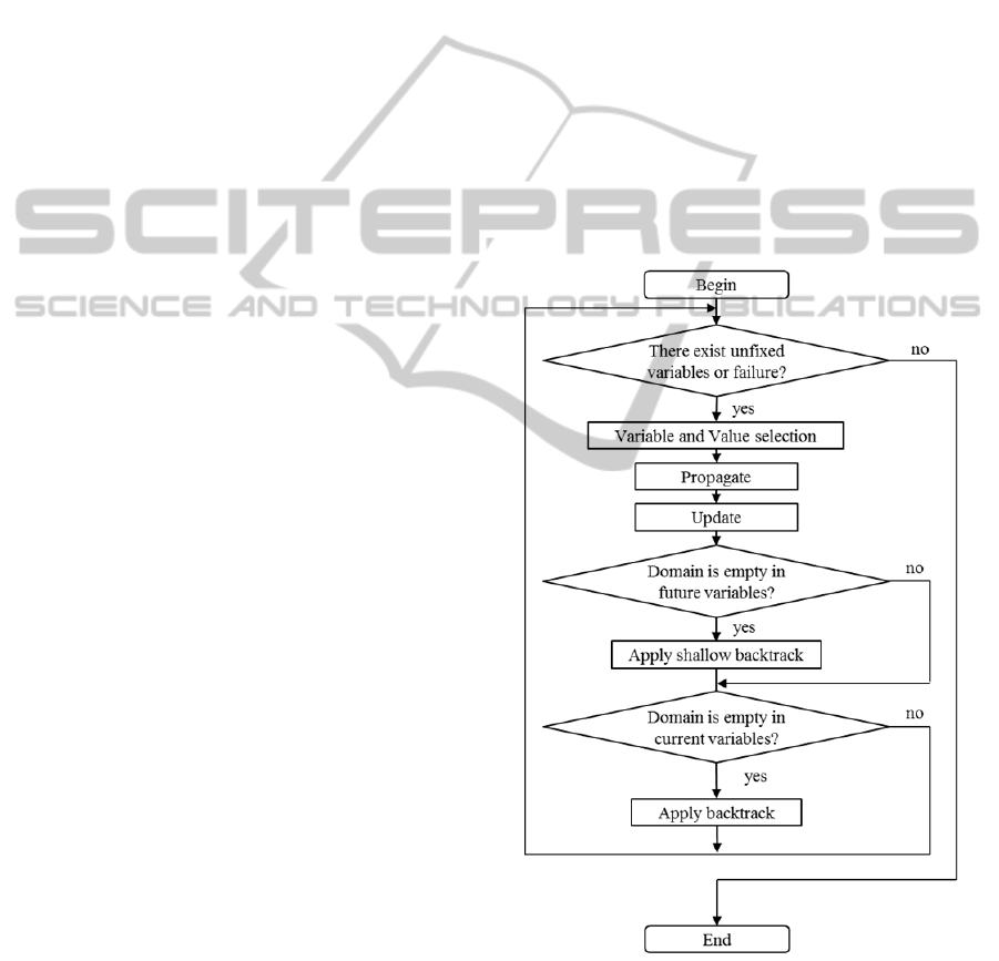
Figure 1: A general algorithm for solving optimization
problems under the CP framework.
The most used approach to solve CSP and
optimization problems under CP is to combine a
backtracking procedure with filtering techniques in
SolvingOpen-PitLong-TermProductionPlanningProblemswithConstraintProgramming-APerformanceEvaluation
71

the form of constraint propagation. Constraint
propagation attempts to delete from domains the
values that do not lead to any solution in order to
accelerate the exploration. The constraint
propagation is performed by validating a consistency
property on the constraints of the problem; the most
used one is the arc-consistency (Soto et al., 2014).
Figure 1 illustrates a general procedure for
solving optimization problems under the CP
framework. The idea is to generate partial solutions
to be verified backtracking when inconsistencies are
detected until a result is encountered. The first step
is to select the variable and its corresponding value
to generate a potential solution to be verified. Then,
the propagation attempts to delete the unfeasible
values. The update instruction is responsible for
storing the best optimum value reached at this time.
Finally two conditions perform backtracks. The
classic backtrack comes back to the most recently
tested variable that has still chance to reach a
solution. A shallow backtrack jumps to the next
value available from the domain of the current
variable.
3 PROBLEM FORMULATION
In this section we formulate the Open-Pit Long-
Term Production Planning Problem. We proceed by
firstly stating the notation followed by the
mathematical model.
3.1 Page Setup
Indices and sets
: time period index ∈1,2,…,.
: set of periods.
: time period index ∈1,2,…,.
: set of blocks.
: index of a block considered for
extraction.
Parameters
: net present value obtained from
mining block in period .
: block grade, which is defined as a
random constant.
: The total amount of ore in block .
: The total amount of waste in block
.
: The maximum material,
including waste and ore, to be mined in
period .
: The minimum material, including
waste and ore, to be mined in period .
: The maximum amount of ore to
be mined in period .
: The minimum amount of ore to be
mined in time .
: The maximum average grade of
material to be processed in time .
: The minimum average grade of
material to be processed in time .
: Discount rate in each period.
: Selling price of metal unit in time .
: Selling cost of metal unit in time .
: Total metal recovery.
: Unit processing cost of ore in time .
: Mining cost of metal unit in time .
: Mining cost of waste material in
time .
: Total number of blocks overlaying a
block.
Variables
: a binary decision variable which is set
to 1 if the block is mined, 0 otherwise.
3.2 Mathematical Model
The Open pit mining long-term scheduling problem
aims at correctly selecting the blocks to be mined in
order to maximize the total profit from the process in
a given period of time. The corresponding objective
function of the problem is depicted below, where
is computed by Eq. 2.
1
1
1
2
The objective function is subjected to several
constraints. For instance, the average grade of the
material sent to the mill must respect given upper
(
) and lower bounds (
). This constraint is
known as grade blending constraint.
∑
∑
3
∈ 1,2,…,
The total tons of material to be exploited are
restricted by processing and mining capacities. The
amount of ore to be processed in each period must
respect the given upper (
) and lower bounds
(
) as stated in Eq. 4. Likewise, the total
ICSOFT-EA2014-9thInternationalConferenceonSoftwareEngineeringandApplications
72
material mined, involving ore and waste, is bounded
by
and
as stated in Eq. 5.
4
∈ 1,2,…,
5
∈ 1,2,…,
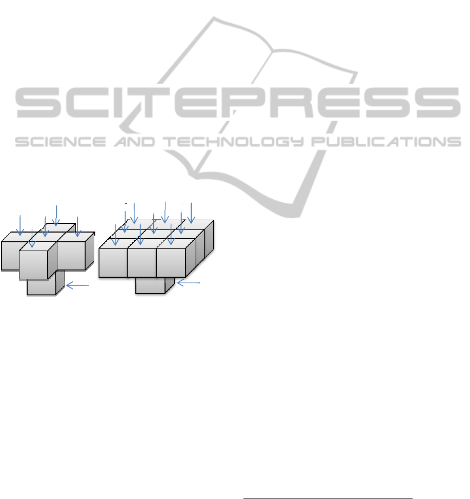
Eq. 6 ensures that all predecessor blocks of a
block must be completely mined in order to have
access and be able to mine the block . This is
commonly represented as a cone model as illustrated
in Figure 2. Finally Eq. 7 guarantees that any block
is mined only once.
0
6
∈
1,2,…,
,∈
1,2,…,
1 ∈ 1,2,…,7
Figure 2: Cone model.
4 EXPERIMENTS
We have performed a set of experiments by using 36
instances of different size in order to compare the
performance of the seven CP solvers. The
experiments have been performed on an Intel Core
i5 with 6 Gb RAM running Windows 7. The
description of solvers and instances is detailed in
tables 1, 2, and 3, respectively. For each instance,
we provide number of periods (), number of blocks
(), number of precedence,
,
,
,
,
, and
. For space reasons,
,
, and
for each block are not included,
but provided in data sets available at
http://inf.ucv.cl/~rsoto/OPM.html.
The results in terms of solving time are depicted
in table 4 and 5. Bold font is used for the best
solving time in each instance, and 10:00:00.000
means that no solution was reached after 10 hours of
running time. The summary of results is depicted in
table 6, which considers as indicators: average
solving time for the complete set of instances
(Avg.), the difference w.r.t the best average solving
time (∆), the standard deviation (), the number of
times the solver achieved the best time for a given
instance (1
st
place), the second best time (2
nd
place),
and the third best time (3
rd
place).
The results illustrate that Gecode, MiniZinc, and
Mzn-g12cpx exhibit the best performance by far.
Gecode achieves the best average solving time close
to the performance of MiniZinc, and Mzn-g12cpx.
Likewise, Mzn-g12cpx obtained 20 first places,
Gecode obtained 13 first places, and MiniZinc 2 first
places. The second places are also taken by these
solvers, MiniZinc taking 21, Gecode 14, and Mzn-
g12cpx only 1. Finally, MiniZinc takes 13 third
places, Mzn-g12cpx takes 8, and Gecode takes 9.
The better performance exhibited by those solvers
with respect to its competitors can be explained by
different reasons. Gecode is a fast solver specially
tuned via efficient propagators for solving this kind
of problems
1
. MiniZinc is rather a modeling
language than a solver, but its default solver is also
very efficient sharing several solving, search, and
filtering features with Gecode. Mzn-g12cpx is a
recent solver based on the lazy clause LazyFD
solver. A lazy clause solver is a hybrid combining
CP and SAT. The idea is to mimic a domain
propagation engine by mapping propagators into
SAT clauses. As a result, we obtain reduced search
by nogood creation, and effective autonomous
search. This leads normally to a faster solving
process.
On the contrary, Mzn-g12fd is a finite domain
solver mostly oriented to satisfaction problems and
perhaps not specially tuned for optimization
problems.
Mzn-g12fdlp, which is the linear programming
version of Mzn-g12fd, slightly improves the results,
but the solving times reached remain quite far from
the best ones. Finally, Choco is a well-known solver
including state-of-the-art CP solving technology but
also rather devoted to constraint satisfaction than
optimization.
1
See results of different competitions at http://www.geco
de.org/
2
1
3
5
4
6
10
4
2
5
6
7
1
9
3
8
SolvingOpen-PitLong-TermProductionPlanningProblemswithConstraintProgramming-APerformanceEvaluation
73

Table 1: Solver Description.
MiniZinc
It is a state-of-the-art high level CP
modeling language that can be
interfaced with several solvers via the
FlatZinc low-level solver input
language. For the experiments, we
employ the default solver for
MiniZinc.
Flatzinc
FlatZinc is the interface of MiniZinc
to derive models to target solvers. For
the experiments, we employ the
default solver for FlatZinc.
Mzn-g12cpx
It is the successor of the LazyFD
solver (lazy clause generation)
involving Constraint Programming
with eXplanations.
Mzn-g12fd
It is the finite domain solver of the
G12 project, to be used with the
MiniZinc modeling language.
Mzn-g12fdlp
It is the linear programming solver of
the G12 project, to be used with the
MiniZinc modeling language.
Choco
It is another state-of-the-art CP solver
implemented on top of Java. It is built
on a event-based propagation
mechanism with backtrackable
structures.
Gecode
It is a well-known CP solver,
implemented as a C++ library. It can
also be interfaced to several languages
such as MiniZinc, Alice, Ruby, and
Lisp.
Table 3: Lower and upper bounds for , per periods,
for all instances.
t1
2000 0 200
t2
2000 0 20000
t3
200000 0 20000
t4
200000 0 200000
t5
200000 0 200000
t6
200000 0 20000
t7
200000 0 20000
Table 2: Instance Description.
Instance
Precedences
1 3 27 98
2 5 27 98
3 7 27 98
4 3 36 140
5 5 36 140
6 7 36 140
7 3 45 182
8 5 45 182
9 7 45 182
10 3 48 200
11 5 48 200
12 7 48 200
13 3 54 224
14 5 54 224
15 7 54 224
16 3 60 260
17 5 60 260
18 7 60 260
19 3 64 300
20 5 64 300
21 7 64 300
22 3 80 390
23 5 80 390
24 7 80 390
25 3 90 416
26 5 90 416
27 7 90 416
28 3 96 480
29 5 96 480
30 7 96 480
31 3 120 624
32 5 120 624
33 7 120 624
34 3 150 832
35 5 150 832
36 7 150 832
Table 4: Lower and upper bounds for , and per
periods, for all instances.
t1
0 0.5 0
t2
0 5 0
t3
0 5 0
t4
0 5 0
t5
0 5 0
t6
0 0.5 0
t7
0 0.5
ICSOFT-EA2014-9thInternationalConferenceonSoftwareEngineeringandApplications
74

Table 5: Solving times of the seven tested solvers for instances 1 to 30 using the hh:mm:ss format. Part 1.
Instance MiniZinc Flatzinc Mzn-g12cpx Mzn-g12fd Mzn-g12fdlp Choco Gecode
2
00:00:00.150
00:00:00.812 00:00:00.930 00:00:02.040 00:00:01.850 00:00:01.280 00:00:00.169
2
00:00:12.997
00:01:00.980 00:02:16.290 00:01:21.120 00:01:11.950 00:01:10.360 00:00:13.043
3 00:03:50.798 00:14:55.507 00:13:13.350 00:15:39.960 00:16:04.700 00:17:04.000
00:03:44.042
4 00:00:03.635 00:00:22.105 00:00:26.360 00:00:23.070 00:00:20.290 00:00:34.540
00:00:02.694
5 00:12:40.846 00:48:20.136 01:40:26.190 00:49:18.220 00:43:28.680 01:07:13.220
00:12:37.014
6 10:00:00.000 10:00:00.000 10:00:00.000 10:00:00.000 10:00:00.000 10:00:00.000 10:00:00.000
7 00:00:00.560 00:00:03.681 00:00:01.770 00:00:03.990 00:00:03.610 00:00:04.401
00:00:00.548
8 00:02:29.646 00:10:36.109 00:05:20.740 00:10:32.120 00:10:17.210 00:12:03.390
00:02:13.807
9 01:58:58.975 07:40:50.599
01:29:02.750
07:38:07.250 07:30:34.710 08:45:14.445 01:59:26.708
10 00:00:00.220
00:00:00.015
00:00:00.500 00:00:02.030 00:00:01.770 00:00:02.710 00:00:00.271
11 00:01:08.555 00:05:22.735
00:00:11.530
00:05:17.390 00:04:54.750 00:05:22.110 00:01:12.042
12 00:16:27.507 00:53:22.070
00:00:46.120
00:56:47.420 00:56:30.670 01:07:10.120 00:22:02.862
13 00:00:00.411 00:00:02.824 00:00:00.630 00:00:03.400 00:00:03.410 00:00:03.004
00:00:00.390
14 00:00:56.978 00:04:19.585
00:00:10.010
00:04:29.830 00:03:44.840 00:04:54.403 00:01:01.748
15 00:16:59.469 01:16:28.910
00:00:48.780
01:24:09.280 01:10:18.450 01:15:40.358 00:15:58.783
16 00:00:04.884 00:00:25.412 00:00:14.000 00:00:23.690 00:00:23.530 00:00:23.710
00:00:04.415
17 01:01:42.276 04:15:41.200 04:53:15.860 04:03:15.000 03:43:18.280 10:00:00.000
01:00:33.329
18 10:00:00.000 10:00:00.000 10:00:00.000 10:00:00.000 10:00:00.000 10:00:00.000 10:00:00.000
19 00:00:00.150 00:00:00.765 00:00:00.800 00:00:01.100 00:00:01.010 00:00:02.030
00:00:00.143
20 00:00:09.617 00:00:43.010 00:00:31.910 00:00:43.630 00:00:41.910 00:01:01.520
00:00:09.604
21 00:01:10.816 00:06:21.000 00:01:57.930 00:06:22.240 00:06:06.300 00:09:03.706
00:01:08.862
22 00:00:16.200 00:01:19.014
00:00:12.740
00:01:19.540 00:01:12.000 00:01:38.060 00:00:16.192
23 03:40:37.626 10:00:00.000
01:11:47.810
10:00:00.000 10:00:00.000 10:00:00.000 03:32:05.568
24 10:00:00.000 10:00:00.000 10:00:00.000 10:00:00.000 10:00:00.000 10:00:00.000 10:00:00.000
25 00:00:00.812 00:00:04.601 00:00:00.771 00:00:04.640 00:00:04.910 00:00:05.010
00:00:00.770
26 00:02:44.479 00:10:14.520
00:00:18.270
00:10:17.310 00:09:40.130 00:10:36.211 00:02:37.258
27 00:31:02.560 02:09:37.945
00:00:47.930
02:06:37.440 02:05:32.460 02:31:24.025 00:30:35.024
28 00:00:00.906 00:00:05.133
00:00:00.750
00:00:05.440 00:00:05.070 00:00:05.457 00:00:00.894
29 00:01:34.900 00:05:27.212
00:00:10.480
00:05:33.400 00:05:03.880 00:05:33.007 00:01:33.349
30 00:30:43.134 02:15:08.105
00:01:01.720
02:48:42.800 02:44:18.000 02:58:12.070 00:31:12.581
5 CONCLUSIONS
In this paper, we have solved the open-pit long-term
production planning problem by using constraint
programming. This problem aims at maximizing the
net present value of the extracted ore from the
mining operation by considering limited processing
plant and mining capacity as well as slope and grade
blending constraints. We have solved this problem
by means of seven well-known CP solvers:
MiniZinc, Mzn-g12cpx, Gecode, Flatzinc, Mzn-
g12fd, Mzn-g12fdlp, and Choco. MiniZinc, Mzn-
g12cpx, and Gecode obtained the best results, which
can be explained by different reasons such as the
incorporation of efficient propagators, and state-of-
the-art search and filtering techniques.
As future work, we expect to study additional
variants of this problem in order to solve them with
constraint programming or related complete and
SolvingOpen-PitLong-TermProductionPlanningProblemswithConstraintProgramming-APerformanceEvaluation
75

Table 6: Solving times of the seven tested solvers for instances 31 to 36 using the hh:mm:ss format. Part 2.
Instance MiniZinc Flatzinc Mzn-g12cpx Mzn-g12fd Mzn-g12fdlp Choco Gecode
31 00:00:01.261 00:00:06.224
00:00:01.010
00:00:06.760 00:00:06.140 00:00:06.210 00:00:01.262
32 00:02:17.578 00:08:07.190
00:00:11.260
00:08:11.050 00:07:46.920 00:08:49.040 00:02:08.285
33 00:35:49.456 02:37:20.354
00:00:55.500
02:39:53.180 02:37:34.020 02:57:41.408 00:32:59.947
34 00:00:00.676 00:00:03.494 00:00:01.020 00:00:03.420 00:00:03.420 00:00:03.588
00:00:00.595
35 00:04:12.895 00:14:03.637
00:00:16.040
00:14:04.330 00:13:31.680 00:14:22.753 00:03:54.553
36 01:00:00.734 02:41:58.363
00:00:44.660
02:48:25.340 02:49:57.390 03:05:42.428 00:50:05.400
28 00:00:00.906 00:00:05.133
00:00:00.750
00:00:05.440 00:00:05.070 00:00:05.457 00:00:00.894
29 00:01:34.900 00:05:27.212
00:00:10.480
00:05:33.400 00:05:03.880 00:05:33.007 00:01:33.349
30 00:30:43.134 02:15:08.105
00:01:01.720
02:48:42.800 02:44:18.000 02:58:12.070 00:31:12.581
31 00:00:01.261 00:00:06.224
00:00:01.010
00:00:06.760 00:00:06.140 00:00:06.210 00:00:01.262
32 00:02:17.578 00:08:07.190
00:00:11.260
00:08:11.050 00:07:46.920 00:08:49.040 00:02:08.285
33 00:35:49.456 02:37:20.354
00:00:55.500
02:39:53.180 02:37:34.020 02:57:41.408 00:32:59.947
34 00:00:00.676 00:00:03.494 00:00:01.020 00:00:03.420 00:00:03.420 00:00:03.588
00:00:00.595
35 00:04:12.895 00:14:03.637
00:00:16.040
00:14:04.330 00:13:31.680 00:14:22.753 00:03:54.553
36 01:00:00.734 02:41:58.363
00:00:44.660
02:48:25.340 02:49:57.390 03:05:42.428 00:50:05.400
Table 7: Summary of performance.
MiniZinc Flatzinc Mzn-g12cpx Mzn-g12fd Mzn-g12fdlp Choco Gecode
Avg. 00:19:02.570 01:05:31.917 00:17:44.134 01:06:40.831 01:04:56.483 01:22:28.139
00:17:08.711
∆
00:01:53.859 00:48:23.206 00:00:35.423 00:49:32.120 00:47:47.772 01:05:19.428 00:00:00.000
00:44:50.159 02:16:14.323 00:55:37.507 02:16:16.958 02:14:44.799 02:48:26.598 00:43:20.211
1
st
place 2 1
20
0 0 0 13
2
nd
place
21
0 1 0 0 0 14
3
rd
place
13
3 8 0 3 0 9
incomplete search techniques. Another interesting
further work would be the introduction of
autonomous search in the solving process. As
detailed in (Crawford et al., 2013, Monfroy et al.,
2013, Soto et al., 2013), the incorporation of
autonomous search in a CP search engine can clearly
speed up the resolution, especially in the presence of
harder instances.
ACKNOWLEDGEMENTS
Ricardo Soto is supported by grant
CONICYT/FONDECYT/INICIACION/ 11130459,
Broderick Crawford is supported by Grant
CONICYT/FONDECYT/1140897.
REFERENCES
Ahuja, R. K, Magnanti, T. L., Orlin, J. B. Network flows,
1993. Theory, Algorithms, and Applications. Prentice
Hall, Englewood.
Boland, N., Dumitrescu, I., Froyland, G., Gleixner, A.,
2009. LP-based disaggregation approaches to solving
the open pit mining production scheduling problem
with block processing selectivity. Computers &
Operations Research, 36 (4), pp. 1064–1089.
Bley A., Boland, N., Fricke, C., Froyland, G., 2010. A
strengthened formulation and cutting planes for the
ICSOFT-EA2014-9thInternationalConferenceonSoftwareEngineeringandApplications
76

open pit mine production scheduling problem.
Computers & OR 37 (9), pp. 1641-1647.
Caccetta, L., Hill, S., 2003. An application of branch and
cut to open pit mine scheduling. Journal of Global
Optimization, 27 (2–3), pp. 349–365.
Chanda, E.K.C., Dagdelen, K., 1995. Optimal blending of
mine production using goal programming and
interactive graphics systems, International Journal of
surface Mining, Reclamation and the Environment,
Vol. 9, pp. 203-208.
Chicoisne, R., Espinoza, D., Goycoolea, M., Moreno E.,
Rubio E., 2012. A New Algorithm for the Open-Pit
Mine Production Scheduling Problem. Operations
Research 60 (3), pp. 517-528.
Crawford, B., Soto, R., Monfroy, E., Palma, W., Castro,
C., Paredes, F., 2013. Parameter tuning of a choice-
function based hyperheuristic using particle swarm
optimization. Expert Syst. Appl. 40 (5), pp. 1690-1695.
Crawford, B., Soto, R., Monfroy, E., Castro, C., Palma,
W., Paredes F, 2013. A hybrid soft computing
approach for subset problems Mathematical Problems
in Engineering, Vol. 2013, Article ID 716069, 12
pages.
Denby, B., Schofield, D., 1994. Open-pit design and
scheduling by use of genetic algorithms. Transactions
of the Institution of Mining and Metallurgy, Section A:
Mining Industry, 103, A21–A26.
Espinoza, D., Goycoolea, M., Moreno, E., Newman, A,
2012. MineLib: A Library of Open Pit Mining
Problems. Ann. Oper. Res. 206 (1), pp. 91-114.
Lamghari, A., Dimitrakopoulos, R, 2012. A diversified
Tabu search approach for the open-pit mine
production scheduling problem with metal uncertainty.
European Journal of Operational Research 222 (3),
pp. 642-652.
Gholamnejad, J., Osanloo, M., Karimi, B., 2006. A
Chance-Constrained Programming Approach for Open
Pit Long-Term Production Scheduling in Stochastic
Environments. The Journal of the South African
Institute of Mining and Metallurgy, Vol. 106, pp.105-
114.
Gholamnejad, J., Osanloo, M., Khorram, E, 2008. A
Chance Constrained Integer Programming Model for
Open Pit Long-Term Production Planning.
International Journal of Engineering Transactions A:
Basics (21) 4, pp. 407-418.
Marcotte, D., Caron, J., 2013. Ultimate open pit stochastic
optimization. Computers & Geosciences Vol. 51, pp.
238-246.
Monfroy, E., Castro, C., Crawford, B., Soto, R., Paredes,
F., Figueroa, C., 2013. A reactive and hybrid
constraint solver. J. Exp. Theor. Artif. Intell. 25 (1),
pp. 1-22.
Pizarro, P., Rivera, G., Soto, R., Crawford, B., Castro, C.,
Monfroy, E., 2011. Constraint-Based Nurse Rostering
for the Valparaíso Clinic Center in Chile. In:
Stephanidis, C. (ed.) Posters, HCII 2011, Part II.
CCIS, vol. 174, pp.448-452, Springer.
Ramazan, S., 2007. The new Fundamental Tree Algorithm
for production scheduling of open pit mines. European
Journal of Operational Research 177(2), pp.1153-
1166.
Soto, R., Crawford, B., Galleguillos, C., Monfroy, E.,
Paredes, F, 2013. A hybrid AC3-tabu search algorithm
for solving Sudoku puzzles. Expert Syst. Appl. 40(15),
pp. 5817-5821.
Soto, R., Crawford, B., Misra, S., Palma, W., Monfroy, E.,
Castro, C., Paredes, F., 2013. Choice functions for
autonomous search in constraint programming: GA vs.
PSO. Tehnicki Vjesnik. Vol. 20(3), pp. 525-531.
Soto, R., Crawford, B., Misra, S., Monfroy, E., Palma, W.,
Castro, C., Paredes, F., 2014. Constraint Programming
for optimal design of architectures for water
distribution tanks and reservoirs: a case study.
Tehnicki Vjesnik. Vol. 21(1).
Soto, R., Kjellerstrand, H., Duran, O., Crawford, B.,
Monfroy, E., Paredes, F., 2012. Cell formation in
group technology using constraint programming and
Boolean satisfiability. Expert Syst. Appl. 39(13), pp.
11423-11427.
Zhang, M., 2006. Combining genetic algorithms and
topological sort to optimize open-pit mine plans. In
proceedings of the 15th mine planning and equipment
selection, pp. 1234–1239.
SolvingOpen-PitLong-TermProductionPlanningProblemswithConstraintProgramming-APerformanceEvaluation
77
