A Generalization of the CMA-ES Algorithm for Functions with Matrix
Input
Simon Konzett
Faculty of Mathematics, University of Vienna, Oskar-Morgenstern-Platz 1, Vienna, Austria
Keywords:
Evolutionary strategies, Evolutionary algorithms, Adaptations, High-dimensional, covariance matrix, Muta-
tion distribution, Self-adaptation.
Abstract:
This paper proposes a novel modification to the covariance matrix adaptation evolution strategy (CMA-ES)
introduced by (Hansen and Ostermeier, 1996) under a special problem setting. In this paper the case is con-
sidered when the function which has to be optimized takes a matrix as input. Here an approach is presented
where without vectorizing directly matrices are sampled and column and row-wise covariance matrices are
adapted in each iteration of the proposed evolution strategy to adapt the mutation distribution. The method
seems to be able to capture correlations in the entries of the considered matrix and adapt the corresponding
covariance matrices accordingly. Numerical tests are performed on the proposed method to show advantages
and disadvantages.
1 INTRODUCTION
Evolution strategies are used to minimize non-linear
objective functions mapping usually a subspace X ⊆
R
n
to R . The iterative strategy is to select good points
and then variate these points in the most promising
way to evolve towards a population of points with
higher quality. Selection is done by comparing func-
tion values of the points in each generation. Variation
means suitable recombination of the population found
so far and to mutate these points to gain more insight.
Mutation can simply mean adding normally dis-
tributed random vectors but often more sophisticated
methods are necessary. Mostly the mutation distri-
bution is characterized by a covariance matrix which
should reflect shape and size of the distribution. Sev-
eral approaches have been proposed to adapt these co-
variance matrices in a promising way. One of the first
ideas proposed is by (Schwefel, 1977). However in
this work a modification of the CMA-ES (Covariance
Matrix Adaption Evolution Strategy) by (Hansen and
Ostermeier, 1996), (Hansen, 1998) and (Hansen and
Ostermeier, 2001) is proposed. The CMA-ES collects
information about successful search steps and stores
this information in so-called evolution paths. The
gained information is used to adapt the covariance
and to slowly derandomise the mutation distribution.
Until now there have been many modifications of
the CMA-ES proposed as in (Jastrebski and Arnold,
2006), (Igeland et al., 2007), (Igel et al., 2006) and
many more.
A modification of the CMA-
ES is proposed concerning functions
f : R
n×m
→ R with matrices as input. This
kind of problem appeared during my research. In
particular the task was to determine suitable param-
eter matrices for a state space model. Obviously
the original CMA-ES method can treat this kind of
problem by just vectorizing the input matrix although
the dimension of such a problem gets quite high soon
for reasonably large matrices. In higher dimensions
the original CMA-ES method need large covariance
matrices to characterize the mutation distribution
and as a result the adaptation for these covariance
matrices should be done carefully and slowly. Same
as in the original CMA-ES the new method will make
use of past successful steps and adapts covariance
matrices related to the rows respectively columns of
the matrix valued mutation distribution. The matrices
to adapt in my proposed method are much smaller
and so on we hope that the method is more flexible
and faster in certain cases.
The paper is from now on organised as in the next
section the original CMA-ES is briefly discussed as
in (N. Hansen, 2011). Then in section 3 the proposed
modification of the CMA-ES is described. Section 4
then shows some computational results and section 5
gives a short review and conclusion.
337
Konzett S..
A Generalization of the CMA-ES Algorithm for Functions with Matrix Input.
DOI: 10.5220/0005159703370342
In Proceedings of the International Conference on Evolutionary Computation Theory and Applications (ECTA-2014), pages 337-342
ISBN: 978-989-758-052-9
Copyright
c
 2014 SCITEPRESS (Science and Technology Publications, Lda.)

2 CMA-ES
In this section a brief outline of the CMA-ES is given.
The problem to solve is generally
min
x∈R
n
f(x) (1)
where f is a non-linear real-valued function.
The algorithm needs initially a starting point m
0
∈
R
n
and a characterization of the initial mutation dis-
tribution given by a covariance matrix C
0
∈ R
n×n
and
an initial global step length σ
0
> 0. Then the algo-
rithm in each iteration is the following.
First a new sample of λ > 0 candidate points is
taken
z
k
∼ N (0, I) (2)
y
k
= BDz
k
∼ N (0, C) (3)
x
k
= m+ σy
k
∼ N (m, σ
2
C) (4)
where m is the best point at this time, the matrices B
and D are given by an eigendecomposition of the co-
variance matrix C = BDDB
T
and the value σ > 0 is
the global step length at this time. So one has a set of
sample points { x
k
}
k=1,...,λ
and these points are com-
pared to each other. The indices of the points x
k
, y
k
, z
k
are reordered such that f(x
k
) ≤ f(x
k+1
) and a new
best point is determined by
m = m+ σ
µ
∑
i=1
w
k
y
k
= m+ σhyi
w
(5)
where µ ≤ λ is the parental population size and w
k
are
weights such that better points have more influence on
the adaptation.
Second the global step size control is done
p
σ
= (1− c
σ
)p
σ
+
+
p
c
σ
(2− c
σ
)µ
eff
BD
−1
B
T
hyi
w
(6)
σ = σ· exp

1
d

kp
σ
k
E(N (0, I))
− 1

(7)
where p
σ
is called the conjugate evolution path. The
conjugated evolution path is normalized such that
p
σ
∼ N (0, I) under purely random selection and then
its length is compared with the expected length un-
der purely random selection. For more details about
the normalization and the step length adaptation I ref-
erence to (Hansen and Ostermeier, 1996), (Hansen,
1998), (Hansen and Ostermeier, 2001) or (N. Hansen,
2011). Basically the idea is that if good steps y
k
point
in a similar direction the accumulation of these points
leads to a larger path length kp
σ
k compared with its
expectation


E(N (0, I))


under purely random se-
lection and as a consequence the global step length
σ > 0 shall grow. Similarly if good steps y
k
can-
cel each other out the global step length σ > 0 gets
smaller. The real parameter d > 0 controls how fast
the global step length can change.
The last part in each iteration of the algorithm is
the covariance adaptation,
p
c
= (1− c
c
)p
c
+
p
c
c
(2− c
c
)µ
eff
hyi
w
(8)
C = (1− c
1
− c
µ
)C+
+ c
1
(p
c
p
T
c
) + c
µ
µ
∑
k=1
y
k
y
T
k
. (9)
The evolution path p
c
is accumulated by the non-
normalized successful steps and the covariance ma-
trix C is updated by a rank-oneupdate of the evolution
path p
c
and a rank-µ update of the selected steps y
k
. If
the covariance matrix C is too large to perform eigen-
decompositions then equation (9) can be replaced by
C = (1− c
1
− c
µ
)C+
+ c
1
diag(p
2
c
) + c
µ
diag
µ
∑
k=1
y
2
k
!
(10)
where diag(x) denotes the diagonal matrix with the
vector x in its diagonal and the square of a vector is
meant component-wise here.
The change rates c
σ
, c
c
, c
1
, c
µ
> 0 are assumed to
be chosen appropriately. In general it can be said that
the choice of suitable changing rates is crucial for the
success of the algorithm. Larger change rates allow
better adaptation and fast change but there are restric-
tions due to the finite amount of information which
is gained through selection. If the change rates are
too large the procedure gets random and if they are
too small the system is rigid and adapts too slowly
which slows the algorithm down. A discussion about
suitable choices of these parameters as well as a dis-
cussion about a suitable population λ > 0 size can be
found in (Hansen and Ostermeier, 1996), (Hansen,
1998) and (Hansen and Ostermeier, 2001). The pa-
rameter µ
eff
> 0 is determined such that p
σ
∼ N (0, I)
and p
c
∼ N (0, C) under purely random selection. It
is easy to see that the adaptation of the mutation distri-
bution is based on the path of successful steps usually
called evolution path.
In the next section the procedure is generalized for
matrices instead of vectors as points of the population.
3 A GENERALIZATION FOR
MATRICES
As the outline of the algorithm remains the same first
a matrix distribution and a sampling procedure need
ECTA2014-InternationalConferenceonEvolutionaryComputationTheoryandApplications
338

to be introduced. The random matrix
X ∼ M N (M, U, V) (11)
is is said to be matrix normally distributed where M ∈
R
m×n
, U ∈ R
m×m
and V ∈ R
n×n
. The distribution is
defined by
vec(X) ∼ N (vec(M), V⊗ U) (12)
and for the matrix normal distribution
E(X) = M (13)
E

(X− M)(X− M)
T

= tr(V) · U (14)
E

(X− M)
T
(X− M)

= tr(U) · V (15)
is true and where tr(X) denotes the trace of a quadratic
matrix X. The expression V ⊗ U denotes the Kro-
necker product of two matrices and vec(X) denotes
the vectorization of a matrix X. For more about ma-
trix distributions I refer to (Dawid, 1981). The prop-
erties (14) and (15) and as a consequence the matri-
ces U ∈ R
m×m
and V ∈ R
n×n
can be interpreted as
column-wise and row-wise covariance. The matri-
ces U ∈ R
m×m
and V ∈ R
n×n
have to be real-valued,
symmetric and positive definite. Further the distribu-
tion M N (M, U, V) is sampled easily by
Y = B
u
D
u
XD
v
B
T
v
(16)
where each entry of the matrix X ∈ R
m×n
is stan-
dard normally distributed and U = B
u
D
u
D
u
B
T
u
and
V = B
v
D
v
D
v
B
T
v
are eigendecompositions.
Thus the first step of the algorithm is
Z
k
∼ M N (0, I
m
, I
n
) (17)
Y
k
= B
u
D
u
Z
k
D
v
B
T
v
∼
∼ M N (0, U, V) (18)
X
k
= M+ σY
k
∼
∼ M N (M, σ
2
U, V). (19)
There is to note that
M N (M, σ
2
U, V) = M N (M, U, σ
2
V)
is true.
Next as in the outline of the original
CMA-ES proposed the population points indices are
reordered by their corresponding function values
such that f(X
k
) ≤ f(X
k+1
). So next the best point
M ∈ R
n×n
is updated by
M = M+ σ
µ
∑
i=1
w
k
Y
k
= M+ σhYi
w
. (20)
Next the global step length σ > 0 has to be
adapted. First the conjugate evolution path is updated
p
σ
= (1− c
σ
)p
σ
+
p
c
σ
(2− c
σ
)µ
eff
B
u
hZi
w
B
T
v
(21)
where
hZi
w
=
µ
∑
i=1
w
k
Z
k
(22)
= B
u
D
−1
u
B
T
u
hYi
w
B
v
D
−1
v
B
T
v
(23)
By using the same arguments as in the original CMA-
ES the conjugate evolution path p
σ
is standard nor-
mally distributed in each row and each column un-
der purely random selection and as a consequence
the vectorized evolution path vec(p
σ
) is also standard
normally distributed under purely random selection.
So the global step length σ > 0 is adapted in the same
manner as in the previous section
σ = σ · exp

1
d

kvec(p
σ
)k
E(N (0, I))
− 1

. (24)
The last step in each iteration is again the covari-
ance adaptation. Here both the column-wise and row-
wise covariance matrices have to be adapted. The
equations are
p
c
= (1 − c
c
)p
c
+
+
p
c
c
(2− c
c
)µ
eff
hYi
w
(25)
tr(V) · U = (1− c
1
− c
µ
)tr(V) · U+
+ c
1
(p
c
p
T
c
) + c
µ
µ
∑
k=1
Y
k
Y
T
k
(26)
tr(U) · V = (1− c
1
− c
µ
)tr(U) · V+
+ c
1
(p
T
c
p
c
) + c
µ
µ
∑
k=1
Y
T
k
Y
k
. (27)
Again the accumulation of the evolution path leads to
p
c
∼ M N (M, U, V) under purely random selection
by the same arguments as in the original CMA-ES.
As easily seen the outline of the algorithm is basi-
cally the same as the original CMA-ES but in the last
covariance adaptation step one has to be careful when
updating the left and right covariance matrices. For
reasons of simplicity the system of equations (26) and
(27) is not solved but the values tr(U) and tr(V) are
taken from the previous iteration.
As already mentioned in the beginning in this pro-
posed algorithm the covariance matrices U and V
which characterize the distribution of the mutation
operator have fewer degree of freedom than the co-
variance matrix C in the original CMA-ES. By us-
ing a matrix normal distribution for the mutation dis-
tribution we have
m· (m+ 1) + n · (n+ 1)
2
degrees of
freedom in the covariance matrices U and V as in
the original CMA-ES the covariance matrix C has
m· n· (m· n+ 1)
2
degrees of freedom. So the vec-
torized problem has a lot more degrees of freedom
AGeneralizationoftheCMA-ESAlgorithmforFunctionswithMatrixInput
339

for adaptation. In high dimensions it is suggested to
use the CMA-ES only with diagonal covariance ma-
trices because computing an eigendecomposition in
high dimensions is costly. Then the degree of free-
dom is only m · n any more which is comparable to
m· (m+ 1) + n · (n+ 1)
2
. However using a diagonal
covariance matrix for characterizing the distribution
of the mutation means just considering the variance of
each coefficient. Thus no correlation between differ-
ent coefficients is considered any more and as a con-
sequence it is also not reflected in the mutation distri-
bution. So the benefit of the proposed method should
be that even in high dimensions correlation between
different variables can be identified.
Next the proposed method is tested on some test
functions.
4 NUMERICAL RESULTS
In this section the original CMA-ES method is com-
pared with the here proposed modification. The
CMA-ES method is executed with the change rates
proposed in (N. Hansen, 2011). Here no eigende-
composition of the covariance matrix in the CMA-ES
are computed because the dimension of the consid-
ered problems is to high. So only diagonal covari-
ance matrices are considered in the original CMA-
ES. The changing rates for the here proposed meth-
ods are adapted from the original method. Numerical
tests suggested that the here proposed method benefits
from larger change rates and fewer sampling points in
each iteration.
I compare here two versions of the original the
CMA-ES algorithm with the here proposed modifi-
cation. The algorithm denoted by CMA-ES1 uses the
initially suggested population size λ > 0 in (Hansen
and Ostermeier, 2001) or (N. Hansen, 2011) and the
algorithm denoted by CMA-ES2 uses smaller popula-
tion size λ > 0 in each iteration same as the method
proposed in this paper. The method which is intro-
duced in this paper is denoted by matrix-CMA-ES in
the figures below.
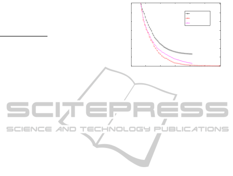
The first test problem which is considered here is
just the spectral norm for matrices,
f
1
(A) = kA− Bk
2
(28)
where B ∈ R
15×20
is a randomly chosen matrix. Ob-
viously the solution for minimizing this function is B
and f (B) = 0. The dimension of the problem by vec-
torizing the matrix A for the original CMA-ES algo-
rithm then is 300. In figure 1 one can easily see that
the here proposed method does not do well solving
1 2 3 4 5 6
x 10
4
0
10
20
30
40
50
60
70
matrixCMA−ES
CMA−ES1
CMA−ES2
Figure 1: Performance of matrix-CMA-ES compared with
CMA-ES1 and CMA-ES2 on the function f
1
. Shown is on
the y-axis the current best function value and on the x-axis
the number of function evaluations at this time.
this problem. As the algorithm continues the progress
gets smaller and smaller. In contrary the original
CMA-ES method works quite good and is able to
solve the problem in a reasonable time. The reason
for the bad behaviour is that there is no linear correla-
tion between different variables to capture and so the
original CMA-ES algorithm where only the variances
of each entry are adapted does a lot better. The be-
haviour for other kind of norm operators is very simi-
lar.
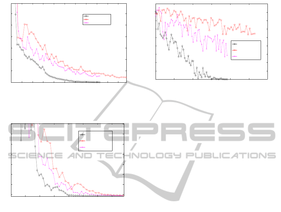
The second problem that is considered is
f
2
(A) = kC· (A− B) · Dk
∞
(29)
where B ∈ R
15×20
, C ∈ R
6×15
and D ∈ R
20×5
are
randomly chosen matrices. The optimal solution
value is again f = 0 but the problem has no unique so-
lution. The dimension of the problem by vectorizing
the matrix A for the original CMA-ES algorithm then
is again 300. This problem obviously has some linear
correlation added by the matrices C and D. In figure
2 one can see that the here proposed method performs
a lot better than the original CMA-ES method. The
reasoning for the better performance is that the modi-
fied procedure is capable of covering the linear struc-
ture of the problem as the original CMA-ES struggles
to do that. The original CMA-ES method even gets
random after some time where no real progress with
respect to the function value can be seen.
The third function numerical tests were performed
on is
f
3
(A) = k(A− B)k
2
+ k(A− C)k
2
(30)
where B ∈ R
15×20
and C ∈ R
15×20
are randomlycho-
sen matrices. The dimension of the problem by vec-
torizing the matrix A for the original CMA-ES al-
gorithm then is again 300. Although the third prob-
ECTA2014-InternationalConferenceonEvolutionaryComputationTheoryandApplications
340

0 0.5 1 1.5 2 2.5 3 3.5 4 4.5 5
x 10
4
0
50
100
150
200
250
300
matrixCMA−ES
CMA−ES1
CMA−ES2
Figure 2: Performance of matrix-CMA-ES compared with
CMA-ES1 and CMA-ES2 on the function f
2
. Shown is on
the y-axis the current best function value and on the x-axis
the number of function evaluations at this time
0.5 1 1.5 2 2.5 3 3.5
x 10
4
278.025
278.03
278.035
278.04
278.045
278.05
278.055
278.06
matrixCMA−ES
CMA−ES1
CMA−ES2
Figure 3: Performance of matrix-CMA-ES compared with
CMA-ES1 and CMA-ES2 on the function f
3
. Shown is on
the y-axis the current best function value and on the x-axis
the number of function evaluations at this time.
lem looks similar than the first problem the perfor-
mance of the modified algorithm is much better. The
proposed algorithm does not outperform the original
CMA-ES but it is a little better than the original ver-
sions. The reason for the better performance is that
here correlation between the coefficients has to be
captured.
The last function I consider is
f
4
(A) = log(|det(C· (A− B) · D)|+ 1) (31)
where B ∈ R
10×12
, C ∈ R
6×12
and D ∈ R
10×6
are
randomly chosen matrices. This problem has no
unique solution but the minimal function value is
f = 0. In figure 4 one can see that the here pro-
posed method drastically outperforms the conven-
tional methods for this problem. The newly proposed
method adapts better to inner structure of the problem
whereas the conventional algorithms can not adapt to
this structure.
0 1 2 3 4 5 6
x 10
4
0
2
4
6
8
10
12
14
16
18
matrixCMA−ES
CMA−ES1
CMA−ES2
Figure 4: Performance of matrix-CMA-ES compared with
CMA-ES1 and CMA-ES2 on the function f
4
. Shown is on
the y-axis the current best function value and on the x-axis
the number of function evaluations at this time.
5 CONCLUSION
As a conclusion this paper has introduced a modifica-
tion to the many existing CMA-ES algorithms. The
goal was to be able to apply a CMA-ES algorithm
to a function where the input is not a vector but a
matrix without vectorizing this matrix. The method
proposed here gives the possibility to do this and the
paper also investigates the advantages and disadvan-
tages of vectorizing the matrix input when a CMA-
ES algorithm is applied. The problem with vector-
izing matrices for the purpose of optimization with
CMA-ES is that vectorizing even fairly small matri-
ces leads quite fast to a high dimensional problem.
In higher dimensions it is very costly and therefore
unreasonable to perform eigendecompositions all the
time during the algorithm. Therefore linear correla-
tions between the variables can not be captured any
more by the conventional CMA-ES algorithm. The
here proposed method considers covariance matrices
of smaller size and it is therefore no problem to do
this eigendecompositions in each iteration. This re-
sults into a better way of capturing the inner structure
of the considered problem. The disadvantage is the
loss of some degrees of freedom in the characteriza-
tion of the distribution of the mutation operator. If the
characterization of the mutation distribution has too
few degrees of freedom like in the first example in
the previous section the behaviour of the optimization
procedure gets random.
In section 4 where some numerical tests have been
performed one can see that the more complicated the
function to minimize is the better the here proposed
method does work as for the easiest kind of problem
where the inner structure is very smooth the conven-
tional method performs a lot better. The modified al-
AGeneralizationoftheCMA-ESAlgorithmforFunctionswithMatrixInput
341

gorithm also seems to allow larger change rates and
is therefore more flexible in capturing the distribution
of the mutation operator.
The method seems applicable for problems which
are not too smooth and where strong linear correla-
tions have to be captured. It is also imaginable for a
high dimensional problems where the covariance ma-
trix in the conventional CMA-ES is too large to per-
form eigendecompositions to rewrite the vector in the
form of an suitably sized matrix such that linear cor-
relations between the variables can be captured by the
applied method.
In further research methods to overcome the dif-
ficulties when the problems structure is very smooth
have to be found. Here I think it is possible to look at
some other modifications of the CMA-ES algorithm.
Moreover the change rates are crucial to the success
of a CMA-ES algorithm. So finding solid and good
change rates for the algorithm will further improve the
proposed method. In addition more numerical tests
have to be performed.
REFERENCES
Dawid, A. P. (1981). Some matrix-variate distribution the-
ory: notational considerations and a Bayesian appli-
cation. Biometrika, 68(1):265–274.
Hansen, N. (1998). Verallgemeinerte individuelle Schrit-
tweitenregelung in der Evolutionsstrategie. Mensch &
Buch Verlag, Berlin.
Hansen, N. and Ostermeier, A. (1996). Adapting arbitrary
normal mutation distributions in evolution strategies:
The covariance matrix adaptation. In Evolutionary
Computation, 1996., Proceedings of IEEE Interna-
tional Conference on, pages 312–317. IEEE.
Hansen, N. and Ostermeier, A. (2001). Completely deran-
domized self-adaptation in evolution strategies. Evo-
lutionary computation, 9(2):159–195.
Igel, C., Suttorp, T., and Hansen, N. (2006). A compu-
tational efficient covariance matrix update and a (1+
1)-CMA for evolution strategies. In Proceedings of
the 8th annual conference on Genetic and evolution-
ary computation, pages 453–460. ACM.
Igeland, C., Hansen, N., and Roth, S. (2007). Covari-
ance matrix adaptation for multi-objective optimiza-
tion. Evolutionary computation, 15(1):1–28.
Jastrebski, G. and Arnold, D. (2006). Improving evolution
strategies through active covariance matrix adaptation.
In Evolutionary Computation, 2006. CEC 2006. IEEE
Congress on, pages 2814–2821. IEEE.
N. Hansen (2011). The CMA Evolution Strategy: A Tuto-
rial.
Schwefel, H. (1977). Numerische Optimierung von
Computer-Modellen mittels der Evolutionsstrategie.
Birkh¨auser Verlag, Basel.
ECTA2014-InternationalConferenceonEvolutionaryComputationTheoryandApplications
342