3-Dimensional Motion Recognition

by 4-Dimensional Higher-order Local Auto-correlation

Hiroki Mori, Takaomi Kanda, Dai Hirose and Minoru Asada

Department of Adaptive Machine Systems, Graduate School of Engineering, Osaka University, Suita city, Osaka, Japan

Keywords:

4-Dimensional Pattern Recognition, Higher-order Local Auto-correlation, Point Cloud Time Series, Voxel

Time Series, Tesseractic Pattern, IXMAS Dataset.

Abstract:

In this paper, we propose a 4-Dimensional Higher-order Local Auto-Correlation (4D HLAC). The method

aims to extract the features of a 3D time series, which is regarded as a 4D static pattern. This is an orthodox

extension of the original HLAC, which represents correlations among local values in 2D images and can

effectively summarize motion in 3D space. To recognize motion in the real world, a recognition system

should exploit motion information from the real-world structure. The 4D HLAC feature vector is expected to

capture representations for general 3D motion recognition, because the original HLAC performed very well

in image recognition tasks. Based on experimental results showing high recognition performance and low

computational cost, we conclude that our method has a strong advantage for 3D time series recognition, even

in practical situations.

1 INTRODUCTION

Motion recognition has many important applications

in ﬁelds such as video surveillance, robotics, human–

computer interaction, and individual behavior analy-

ses for marketing. Recognition systems should effec-

tively exploit features from the real world that exist in

space and time (4D space).

Most conventional methods for recognizing mo-

tion use the color or intensity time series from 2D im-

ages. However,such images suffer from a light condi-

tion and motion in the depth direction. Motion in 3D

space, rather than motion in depth, must be consid-

ered to solve this difﬁculty with 2D images. However,

there has been little research on the direct application

of 3D time series to the wide variety of motion recog-

nition applications.

In this paper, we propose a 4-Dimensional Higher-

order Local Auto-Correlation (4D HLAC) that can

represent pattern features in point-cloud time series

data and tesseract array data (voxel-time series data).

The concept of HLAC (Otsu and Kurita, 1988) can be

applied to any data array to extract the features of the

pattern. However, the original article on HLAC only

considered 2D image data in which features are char-

acterized by model-free, shift invariance, and additiv-

ity. HLAC can also be applied to 3D array data (Cubic

HLAC, or CHLAC (Kobayashi and Otsu, 2004)) to

handle 3D objects and 2D movies (2D images + time

series). However, only 4D HLAC allows voxel time

series to be directly recognized as a static object con-

sisting of tesseracts in 4D space. We have conducted

two experiments that apply 4D HLAC to human mo-

tion to examine the performance and computational

cost of the method.

The remainder of this article proceeds as follows.

Some related work in the ﬁeld of 3D motion recogni-

tion is discussed in Section 2, and our proposed 4D

HLAC feature is introduced in Section 3. Section 4

describes the experimental setup, and Section 5 com-

pares our results with those from previous research

based on the IXMAS dataset. Finally, we present our

conclusions in Section 6.

2 RELATED WORK

In this section, we summarize related work on 3D mo-

tion recognition. 3D motion recognition is mainly

performed in a multi-camera environment, whereby

the motion of an object is captured by multiple cam-

eras from different perspectives. Previous image fea-

tures can be separated into two categories based on

how many spatial dimensions they use: the raw 2D

images from multiple cameras, or a reconstructed 3D

representation.

223

Mori H., Kanda T., Hirose D. and Asada M..

3-Dimensional Motion Recognition by 4-Dimensional Higher-order Local Auto-correlation.

DOI: 10.5220/0005200602230231

In Proceedings of the International Conference on Pattern Recognition Applications and Methods (ICPRAM-2015), pages 223-231

ISBN: 978-989-758-076-5

 2015 SCITEPRESS (Science and Technology Publications, Lda.)

One approach is to use 2D image processing tech-

niques and features from multi-view cameras, such as

spatiotemporal interest points (Wu et al., 2011) from

2D movies, and silhouette-based features (Cherla

et al., 2008; Chaaraoui et al., 2014). Weinland et al.

(2010) proposed a 3D modeling method that produces

2D image information for recognition. Following fea-

ture extraction, their method does not use 3D recon-

struction in the recognition phase (Weinland et al.,

2010).

Concepts based on 3D analysis tend to extract fea-

tures from 3D data such as point clouds and voxel im-

ages. Previous studies of 3D motion features have

proposed various techniques, such as a layered cylin-

drical Fourier transform around the subject’s vertical

axis (Weinland et al., 2006; Turaga et al., 2008), cir-

cular patterns intersecting the subject’s body on hori-

zontal planes, 4D spatiotemporal interest points (4D-

STIP), and optical ﬂows based on HoG to represent

3D motion (Holte et al., 2012).

Our approach in this paper is based on the idea

of HLAC (Otsu and Kurita, 1988). After HLAC

was applied to pattern recognition in static 2D im-

ages, 3D extensions of HLAC were proposed for the

recognition of 2D movies as spatiotemporal patterns

(Kobayashi and Otsu, 2004) and the recognition and

retrieval of 3D objects (color cubic HLAC, or CCH-

LAC (Kanezaki et al., 2010)). To use CHLAC for 2D

movies, a layered 2D image that changes with time is

considered to represent a 3D object in the spatiotem-

poral domain. This extension from HLAC to CHLAC

inspired the idea of 4D HLAC. A comparison of the

different HLAC variations is shown in Figure 2. In

the next section, we give a deﬁnition of HLAC, de-

scribe its extension to four dimensions, and identify

certain characteristics and theoretical expectations for

4D HLAC.

3 4D HLAC

3.1 Basic Idea of HLAC

The Nth-order auto-correlation function is deﬁned as

h(a

,...,a

) =

f(r) · f (r+ a

) · ... · f(r+ a

)dr,

(1)

where r is a reference vector in an image and a

(i =

1,... , N) are displacement vectors based on r. A fea-

ture x is deﬁned by the order of N and the displace-

ments a

. Therefore, a feature vector consists of all

possible variations of h, with a constraint on the max-

imum size of N and the distance between a and r. Fi-

nally, any equivalent variations are eliminated.

In practical terms, Equation (1) should be dis-

cretized into

h =

∑

...

∑

{z }

I(i,...,l) · I(i+ a

[1],... , l + a

[D]) · ...

· I(i+ a

[1],... , l + a

[D]),

(2)

where I(i,... , j) is a D-dimensional image, meaning

the summation is applied D times. The set of vectors

...a

represents one of the higher-order correlation

patterns. The term a

[·] represents an element of the

vector a

. In light of previous HLAC research (Otsu

and Kurita, 1988; Kobayashi and Otsu, 2004), we as-

sume that the order N is less than or equal to 2, and

the range of the displacement is deﬁned by a local

3 × ··· × 3 region. HLAC masks for 2D images are

shown in Figure 1. One of the patterns for N = 2 is

represented by a

= (1,0),a

= (1, 1) in the top-left

image of Figure 1. If an image I is a binary array, ex-

tracting the HLAC features is a very simple operation

(namely, counting the number of local patterns in I).

3.2 Formulation

We propose 4D HLAC to represent the features of

tesseractic (4D cubic) images in 4D space for pattern

recognition in 3D motion. Conditions for the different

HLAC variants are summarized in Table 1 (N = 0,1,2

and the local 3 × ··· × 3 region for combinations of

HLAC dimensions (2, 3, or 4) and values (gray or

binary)). In most cases, 3D data in one time frame

are provided as a depth image, a voxel image, multi-

view camera images, or point clouds. To extract a 4D

HLAC feature, the data must be transformed into a

voxel image or point clouds. After the time series for

these voxels (or point clouds) have been obtained, the

4D HLAC for 3D motion is deﬁned by the following

equations:

h =

∑

)

· I

+ L

[1],D

+ L

[2],

+ L

[3],D

+ L

[4]) · ...

· I

+ L

[1],D

+ L

[2],

+ L

[3],D

+ L

[4])

(3)

(x,y,z,t) =











1 if a tesseract with vertices

(x,y,z,t),(x+ L

,y,z,t),

...,(x+ L

,y+ L

,z+ L

,t + L

)

includes at least one point.

0 otherwise.

(4)

ICPRAM2015-InternationalConferenceonPatternRecognitionApplicationsandMethods

224

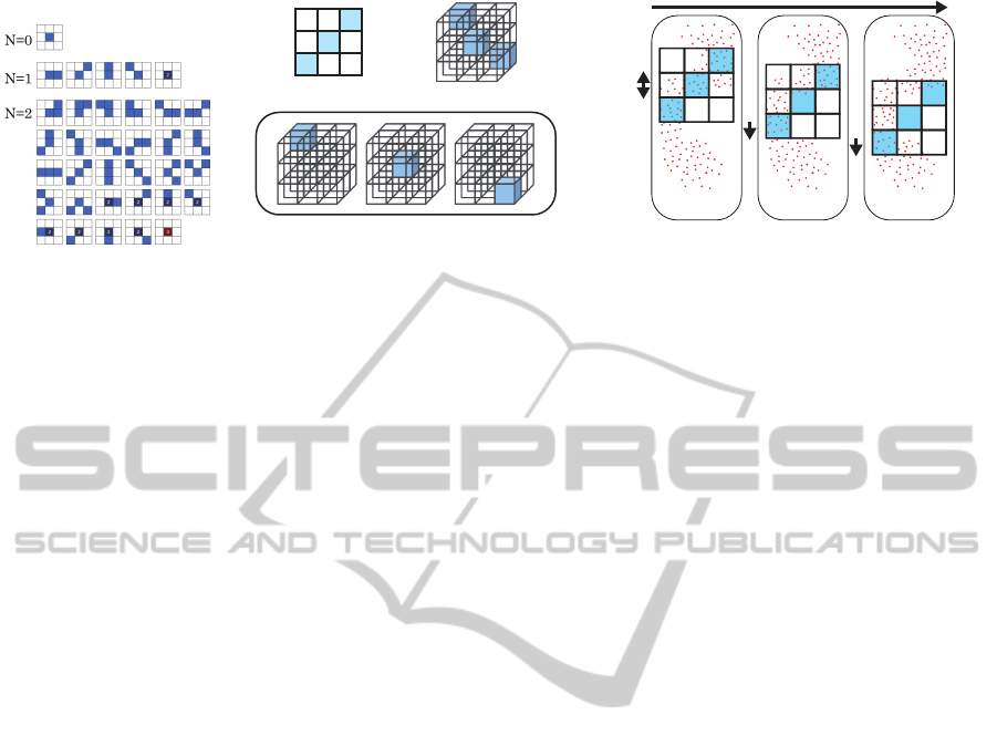
Figure 1: All masks of HLAC

for a gray-scale 2D image.

(b) One of second order CHLAC

masks as a voxel pattern

(a) One of second order HLAC

masks as a pixel pattern

Figure 2: Comparison of HLAC varia-

tions.

Shift D

Integration process

Tesseract edge

length Lx

Feature h=1 h=2 h=2

I (x,y,z,t) I (x+D

,y,z,t) I (x+2D

,y,z,t)

4D 4D 4D

Figure 3: Operation of HLAC from point

clouds.

The extraction of 4D HLAC features is executed ac-

cording to the diagram in Figure 3. The 4D HLAC

parameters are as follows:

x,y,z

: Tesseract edge length [mm] in space.

: Tesseract edge length [ms] in time.

x,y,z

: Shift distance [mm] required to move HLAC

mask patterns in space.

: Shift distance [ms] required to move HLAC

mask patterns in time.

x,y,z

: Analyzed area length [mm] in space.

: Analyzed area duration [ms] in time.

x,y,z

: Number of HLAC summations in space

x,y,z

= ⌊A

x,y,z

⌋).

: Number of HLAC summations in time (M

⌊A

⌋).

In this study, the sampling rates D

and L

were ﬁxed

to 33 [ms]. L

x,y,z

represents the resolution of the pat-

tern. A 4D HLAC feature with small L

x,y,z

describes

the local form and motion in detail, such as the ﬂuc-

tuation of clothes or vibratory movements of a single

body part. A 4D HLAC feature with large L

x,y,z

de-

scribes a holistic form and motion of an object, such

as the coordination of multiple body parts. When the

3D data is ﬁrst provided as a voxel time series, the

point clouds in the theory are equivalent to voxels.

Voxel time series that are transformed from raw

data (e.g., point clouds) may be subjected to tem-

poral subtraction or surface extraction if necessary.

Temporal subtraction is intended to emphasize mo-

tion by deleting motionless objects, and surface ex-

traction ensures that objects ﬁlled by voxels are ac-

counted for, because most of the raw data from 3D

depth sensors are regarded as surface patterns. We

generally need to test whether such preprocessing is

effective for the given purpose.

In this research, rather than gray-scale patterns,

we use binary tesseract patterns of spatiotemporal ar-

rays (these can be constructed from point clouds by

counting the points in one tesseract). We use binary

patterns because the sharp boundaries between ob-

jects and void space are transformed into discriminat-

ing features. This characteristic is useful in many ap-

plications, including human motion recognition. We

suggest that gray-scale 4D HLAC should be used for

certain types of ﬂuid analysis because of its continu-

ous density gradients.

3.3 Characteristics

Analogous to the original HLAC features, 4D HLAC

has the following characteristics:

(a) Model-free. The method does not require any ob-

ject or world model.

(b) Simple Algorithm. The operations of the

method only involve counting local patterns.

ation such as edge extraction. The integration in

the operation of HLAC is expected to eliminate

noise analogously to a low-pass ﬁlter.

(d) Low Computational Cost and Easy Paralleliza-

tion. Counting the patterns is a low-cost oper-

ation. The algorithm is easily parallelized by

arranging the computation of each pattern or

separated target area into one process. The paral-

lelization algorithms are discussed in Section 3.4

The computation time of one recognition and the

efﬁciency of the parallelization are discussed in

Section 5.

(e) Spatiotemporal Shift Invariant. The integra-

tion eliminates the location of the patterns. This

invariance makes the recognition robust.

(f) Additivity. The feature vector, including multiple

objects and their motion, is the sum of all single

feature vectors of the objects and the motions in

the image. In Section 4.2, we exploit this charac-

teristic to count action classes with constant com-

putational load.

3-DimensionalMotionRecognitionby4-DimensionalHigher-orderLocalAuto-correlation

225

Table 1: Number of masks for the HLAC variations.

Name Dimen- Mask size Mask variation

sion Gray Binary

HLAC 2D 3 × 3 35 25

CHLAC 3D 3 × 3 × 3 279 251

4D HLAC 4D 3 × 3 × 3 × 3 2563 2481

(g) High Performance for Pattern Recognition.

We show that the performance of our method is

very high compared to 2D movie methods (Sec-

tion 4.1) and to previous 3D methods (Section

5).

3.4 Implementation

Characteristic (d) ensures that 4D HLAC can be ef-

fectively parallelized. In this research, we implement

4D HLAC on a single core with a sequential program,

a multiple core CPU with OpenMP, and a GPGPU

using CUDA. To parallelize the method, we divide

the computation into that for a single HLAC pattern

and the integrations regarding the time axis. For the

HLAC patterns, we developed 2481 CUDA threads

to compute the local patterns of binary 4D HLAC on

a GPGPU. To avoid redundant computations, we di-

vide the target 4D space along the time axis. When

raw data are provided for a moment t, a partial feature

vector at t − 1 is acquired from the data in three time

frames (t,t − 1,t − 2), and this partial feature vector

is added to a queue. Finally, the queued partial fea-

ture vectors from the time window between t − 1 and

t − 1 − M

are summed, and the oldest partial feature

vector is deleted from the queue. This algorithm re-

duces the computation by a factor of 1/M

, although

the operation is completely equivalent to a one-shot

computation for a target time window.

4 BASIC EXPERIMENT

4.1 Classiﬁcation

4.1.1 Experimental Setup

a In this section, we examine how the 4D HLAC fea-

tures contribute to the recognition of very simple hu-

man arm motions, and compare this to conventional

2D motion analyses. The motion classes for the ex-

amination are very simple arm rotations, as shown in

Figure 4. These are characterized by movement in the

depth and vertical (up-down) directions, so the recog-

nition should exploit information about the location

and velocity of the arm movements in 3D space.

Table 2: Test data in the basic classiﬁcation experiment.

Actors 10

Class of actions 3

Trials of one action 10

by one subject

Frame rate 30 [fps]

Frame size for one trial 250 frames (8.3 [s])

Analyzed duration 20 (666[ms])

of time frame M

Analyzed area A

x,y,z

900×900×900 [mm]

Resolution in 2D images 640 × 480[pixel]

The data were acquired as RGB-D images from a

depth sensor (Microsoft Kinect). The examples of the

data acquired from Kinect is shown in Figure 5. The

images were transformed into 3D voxel time series,

2D intensity image time series, and 2D depth image

time series. Note that 3D voxel data and depth im-

ages are theoretically reversible by interconversion.

We expect that a comparison between them will in-

dicate how the real-world structure in the spatiotem-

poral domain contributes to motion recognition, even

when the structure is only captured from one perspec-

tive.

We set L

x,y,z

= 10, 20, 30, and 50 [mm], L

=33

[ms], and D

x,y,z,t

= L

x,y,z,t

in all analyses. The time

frame was M

= 20 frames. In the classiﬁcation part,

we used Fisher’s Discriminant Analysis (FDA) for di-

mension reduction and the Minimum Distance Clas-

siﬁer. Features were extracted at each point by sliding

the time window, and the classiﬁer assigned one of the

action classes to the current feature.

We applied the CHLAC feature to depth movies

and intensity movies (Figure 6). The backgrounds

were eliminated from these movies based on depth

information. For the CHLAC feature in this exami-

nation, the auto-correlation order was N = 0, 1, 2, and

the range of displacements a

was within a 3× 3 × 3

local region. The 2D image resolution was scaled to

1, 0.5, 0.3, 0.2, and 0.1 times that of the original im-

age. This change of resolution is equivalent to chang-

ing the voxel size. Edge extraction was based on the

Canny Method (Canny, 1986), with parameter values

of 50, 250, or 450. All parameter combinations were

applied to determine the combination that produced

the best result.

We collected the test data for the examination

under the conditions listed in Table 2. The clas-

siﬁcation rate was calculated by leave-one-actor-out

(LOAO) cross-validation, whereby the correct recog-

nition rates for one actor’s actions are calculated after

the recognition system is learned from the other ac-

tors’ actions. Finally, we calculated the average and

ICPRAM2015-InternationalConferenceonPatternRecognitionApplicationsandMethods

226

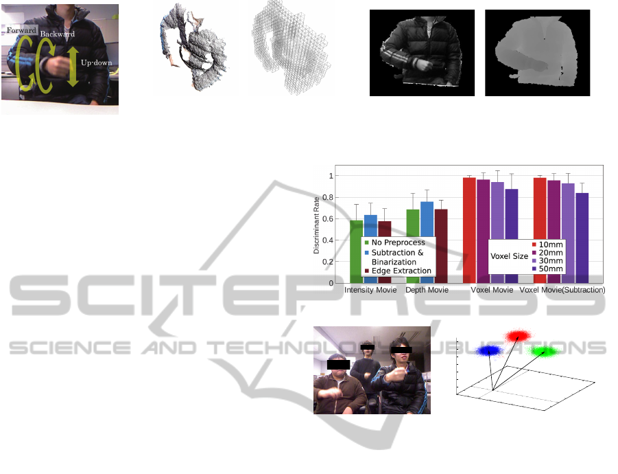
Figure 4: Motion classes

in the basic experiments.

(a) (b)

Figure 5: Data types of 3D movies:

(a) Point cloud data (b) Binary voxel data.

(a) (b)

Figure 6: Images used in the comparative ex-

periment: (a) Intensity image (b) Depth image.

standard deviation of the recognition rates for all ac-

tors.

4.1.2 Results

The experimental results are shown in Figure 7. From

the 4D HLAC experiments, the best classiﬁcation rate

was 98.2% for the smallest voxel size (10 [mm]).

Temporal subtraction before 4D HLAC produced al-

most the same performance as without subtraction.

This implies that 4D HLAC can extract features ap-

propriate to movement.

Using CHLAC, 2D intensity and depth movies

induce worse performance than 3D movies with 4D

HLAC, even when both movies have exactly the same

perspective. The best classiﬁcation rates were 63.5%

for intensity movies and 75.8% for depth movies.

The results from intensity movies are better than the

chance level (33%), but worse than the results from

depth movies and voxel movies. This indicates that

the real-world structure in 3D space is critical for the

recognition, even when only one perspective is used

and the image includes some occlusion.

Although depth movies are supposed to contain

the same information as voxel movies, feature extrac-

tion from depth movies using CHLAC is worse than

that from voxel movies by 4D HLAC. The reasons for

this low performance with depth movies are as fol-

lows:

Boundary Effect. The boundaries between a mov-

ing arm and a body trunk are taken into account,

whereas physically distant body parts do not con-

tribute.

Depth Direction. The motion along the depth axis

in depth movies is represented by the change of

gradient in the depth value. However, temporal

changes in gradient are difﬁcult to capture.

We believe the reasons above can be applied to any

other 2D image descriptors for depth movies.

Figure 7: Results of the discrimination experiment.

Figure 8: Simultaneous

actions by three actors.

-0.02

-0.01

0.01

0.02

0.03

0.04

0.05

0.06

-0.01

0.01

0.02

0.03

0.04

0.05

0.02

0.04

0.06

0.08

0.1

0.12

0.14

Figure 9: The discriminant space

with zero-motion for decomposi-

tion of the three motions.

4.2 Counting

4.2.1 Theory and Experimental Setup

To demonstrate the usefulness of the additivity prop-

erty, we constructed an algorithm to count target mo-

tions with a computational cost that is independent of

the number of actions in the target area.

The HLAC vectors h are interpreted as:

h ≈ n

+ n

+ ... + n

+ ε, (5)

where m

,...,m

are the average feature vectors

of the respective action classes, n

,...,n

are the

number of actions, and ε is a vector of common el-

ements in all classes. The lengths of the decom-

posed vectors n

,...,n

based on the base vec-

tors m

,...,m

represent the number of actions

if the acquired h can be decomposed into vectors

,...,n

To estimate the number of classes, we must cal-

culate the inverse of Equation (5) from h to n =

,...,n

). To estimate the inverse function, we

propose the following algorithm.

3-DimensionalMotionRecognitionby4-DimensionalHigher-orderLocalAuto-correlation

227

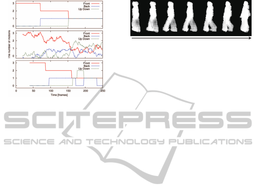
Figure 10: Results of the counting experiment. Top:

Ground truth; Middle: Estimated motion numbers; Bottom:

Discretized estimated motion numbers.

1. Suppress the feature space with all target action

data and common action ε using FDA. The dimen-

sion of the suppressed feature vector is the number

of classes C.

2. Transform the average vectors of action

classes m

,...,m

into the FDA space

ˆm

, ˆm

,..., ˆm

3. Calculate the inverse matrix of

( ˆm

−

ε ˆm

−

ε ... ˆm

−

ε).

4. Estimate the vector of the number of actions.



··· n



= ( ˆm

−

ε ˆm

−

ε .. . ˆm

−

ε)

−1

(6)

where

h is transformed from the feature vector h

into FDA space.

5. Discretize (n

...n

)

using a rounding func-

tion.

We adopt the zero-vector as the common vector ε af-

ter applying temporal subtraction to the voxel time se-

ries; temporal subtraction for an unchanged time se-

ries results in 0. The inversefunction can be estimated

using multiple regression and a pseudoinverse. How-

ever, these methods require training data with all pos-

sible combinations of actions in the learning phase,

whereas the proposed method only requires training

data from one action with one label.

We used the data from the previous experiment to

learn the average class vectors m

, and conducted an

experiment with three actors to estimate the number

of action classes (Figure 8). L

x,y,z

and D

x,y,z

were set

to 30 [mm].

Time

Figure 11: Example of a walking pattern in the voxel time

series of the IXMAS dataset.

4.2.2 Results

The training data in the compressed feature space for

the three motions are shown in Figure 9. The motion

counting results are shown in Figure 10. We calcu-

lated the simple moving averages, and rounded these

to give (n

...n

)

. The results show that the esti-

mated number of motions follows the actual number.

An additional experiment showed that a smaller

voxel size (10 [mm]) produces a worse result. Gener-

ally, smaller voxel sizes are too sensitive to small ir-

relevant motion or measurement noise. For instance,

in this experiment, the third person was further away

from the measuring instrument than in the discrimi-

nant experiment; thus, bigger voxels (30 [mm]) gave

better results.

5 IXMAS DATASET

5.1 Experimental Setup and Method

To compare 4D HLAC to previous 3D motion recog-

nition techniques, we applied the proposed method

to the IXMAS dataset (Weinland et al., 2006). This

dataset has been used for various studies into pattern

recognition in 3D motion. We shall demonstrate the

advantages of our method in terms of recognition per-

formance and computational cost.

The IXMAS dataset consists of multi-view cam-

era movies and voxel time series. The voxel time se-

ries data are applicable to our method (Figure 11).

The multi-view camera system ensures there is no

critical occlusion in the data, unlike in the previous

section. The inside of each object is ﬁlled by voxels,

with the length of each voxel edge estimated to be 30–

40 [mm] (this edge length is not explicitly speciﬁed,

but is not important for this experiment).

To recognize motion in any direction, we generate

additional training data by rotating the original train-

ing data around the vertical axis in 15

◦

steps. Rotation

invariance can be ensured by making a new feature

vector as the sum of all the rotated feature vectors.

ICPRAM2015-InternationalConferenceonPatternRecognitionApplicationsandMethods

228

Table 3: Computational time of 4D HLAC for IXMAS

dataset; M

=20 [frames].

Implementation

Time [ms]

One shot

Queue and sum

CPU (Single thread) 6346 317

CPU (12 threads) 932 46

GPGPU 183 9

(2481 CUDA threads)

CPU: Intel Core i7-3930K 3.2 Hz (6 cores), GPU: GeForce GTX 680 (1536

cores), Memory: 31.4GB, OS: Ubuntu 12.04 64bit.

“One shot” represents

consumed time for the calculation of a HLAC feature vector for 20 frames

at one time.

“Queue and sum” represents the computation time using the

algorithm with a queue of partial feature vectors.

Contrary to our expectation, the results from this op-

eration are almost the same, or slightly worse, than

the strategy with additional rotated training data for

learning and original features for recognition.

When examining the performance of 4D HLAC,

we must evaluate the following conditions for the ex-

traction of features:

Effect of Surface. In most cases, a 3D range sensor

provides information about the object surface. We

utilize the voxel data format with and without sur-

face extraction.

Independent Analysis of Upper and Lower Bodies.

Generally, HLAC eliminates any locations in

which a HLAC pattern occurs, whereas human

whole-body motion consists of independent or

dependent multi-body motion. Independent mo-

tion should be analyzed independently for precise

recognition. We split the analyzed area into the

upper and lower body, divided at the central

horizontal plane. The height of this plane is

deﬁned by the average mid-points of the distance

between the highest and lowest voxels for the

analyzed time frame M

. Under this splitting

condition, the feature vector has 4962 elements

(2481×2).

Detail of Motion. We varied L

x,y,z

to adjust the

granularity of the motion details in order to cor-

rectly capture the coordination among body parts.

We utilize a linear support vector machine (LSVM)

to classify the actions after FDA is applied to the 4D

HLAC feature vectors. The recognition in each trial

is determined by a majority vote of the system recog-

nition in every frame while the system recognizes the

behavior in a frame based on the last 20 frames (M

5.2 Results

Under the above experimental conditions, we ob-

tained the results listed in Table 5. Our method

achieved an optimal recognition rate of 95.5%.

When using the additional data generated by rotat-

ing the original data, the distribution of training sam-

ples from a certain action class forms a closed curve

in the feature space. Regardless of such a non-normal

distribution, the experimental results are good, even

those from the linear classiﬁcation method, because

the feature vectors of actions in the feature space

are signiﬁcantly separated. This indicates that our

method can capture the effective features of actions

from the raw voxel time series.

Table 4 gives the confusion matrix. The most

confusing actions are the hand-waving and head-

scratching actions. Both actions consist of hand shak-

ing movements. The reason for the misrecognition is

that contact between a hand and the head is very difﬁ-

cult to detect, because the local patterns at the contact

points can easily be occluded.

Table 3 gives the computational time needed to

compute the feature for the most effective condition.

The fastest time of 9 [ms] for one time classiﬁcation

was given by GPGPU parallelization, while CPU par-

allelization is also effective (46 [ms]). The classiﬁca-

tion method combining FDA and LSVM takes only

a few microseconds because it consists of only linear

calculations.

To compare our method with previous methods,

the LOAO performanceof some state-of-the-artmeth-

ods is given in Table 6. Although the recognition

rate is a good performance indicator, it is not easy

to compare the recognition rates of each method be-

cause of their different experimental conditions. Ac-

cording to Table 6 and Table 3, our method outper-

forms those previous methods that reported a compu-

tation time, demonstrating that the computational cost

of our method is very competitive.

Among all methods, the performance of our

method is third behind those of Holte et al. (2012)

and Turaga et al. (2008). Neither of these studies re-

ported a computational cost, though Turaga et al. ar-

gued that their method was computationally efﬁcient.

The method of Holte et al. may have a much higher

computational cost than our method, as it relies on a

complicated algorithm to produce the highest recog-

nition rate (100%). Turaga et al. proposed a clas-

siﬁcation method based on statistical manifold learn-

ing with a 3D motion feature (Weinland et al., 2006),

and reported a slightly higher performance rate than

our method. This indicates that our method can be

improved by a further appropriate classiﬁcation tech-

nique.

3-DimensionalMotionRecognitionby4-DimensionalHigher-orderLocalAuto-correlation

229

Table 4: Confusion matrix for IXMAS dataset: mask size L

x,y,z

= 4; average recognition rate = 95.5%; (·) represents the

number of trials recognized as each action class in 36 samples (12 actors × 3 trials).

Recognized Performed actions

actions Check watch Cross arm Scratch head Sit down Get up Turn around Walk Wave hand Punch Kick Pick up

Check watch 94.4(34) 0.0(0) 0.0(0) 0.0(0) 0.0(0) 0.0(0) 0.0(0) 0.0(0) 0.0(0) 0.0(0) 0.0(0)

Cross arm 5.6(2) 100.0(36) 2.8(1) 0.0(0) 0.0(0) 0.0(0) 0.0(0) 2.8(1) 0.0(0) 0.0(0) 0.0(0)

Scratch head 0.0(0) 0.0(0) 97.2(35) 0.0(0) 0.0(0) 0.0(0) 0.0(0) 16.7(6) 0.0(0) 0.0(0) 0.0(0)

Sit down 0.0(0) 0.0(0) 0.0(0) 100.0(36) 0.0(0) 0.0(0) 0.0(0) 0.0(0) 0.0(0) 0.0(0) 2.8(1)

Get up 0.0(0) 0.0(0) 0.0(0) 0.0(0) 100.0(36) 0.0(0) 0.0(0) 0.0(0) 0.0(0) 0.0(0) 0.0(0)

Turn around 0.0(0) 0.0(0) 0.0(0) 0.0(0) 0.0(0) 100.0(36) 5.6(2) 0.0(0) 0.0(0) 0.0(0) 0.0(0)

Walk 0.0(0) 0.0(0) 0.0(0) 0.0(0) 0.0(0) 0.0(0) 88.9(32) 0.0(0) 0.0(0) 0.0(0) 0.0(0)

Wave 0.0(0) 0.0(0) 0.0(0) 0.0(0) 0.0(0) 0.0(0) 0.0(0) 80.6(29) 5.6(2) 0.0(0) 0.0(0)

Punch 0.0(0) 0.0(0) 0.0(0) 0.0(0) 0.0(0) 0.0(0) 0.0(0) 0.0(0) 91.7(33) 0.0(0) 0.0(0)

Kick 0.0(0) 0.0(0) 0.0(0) 0.0(0) 0.0(0) 0.0(0) 2.8(1) 0.0(0) 2.8(1) 100.0(36) 0.0(0)

Pick up 0.0(0) 0.0(0) 0.0(0) 0.0(0) 0.0(0) 0.0(0) 2.8(1) 0.0(0) 0.0(0) 0.0(0) 97.2(35)

Table 5: LOAO recognition rate [%] for IXMAS dataset

with different feature extraction conditions; L

x,y,z

is voxel

size in the IXMAS format.

x,y,z

Whole body Separated into

upper and lower bodies

Filled Surface Filled Surface

1 84.3 % 81.1 % 87.4 % 89.1 %

2 91.2 % 88.1 % 94.4 % 90.7 %

3 90.9 % 91.9 % 94.7 % 92.7 %

4 92.7 % 91.7 % 93.7 % 95.5 %

5 93.4 % 91.4 % 91.9 % 93.2 %

6 92.2 % 92.7 % 90.7 % 90.7 %

Table 6: Comparison with 3D human action recognition ap-

proaches. The results for the LOAO cross-validation were

obtained using the IXMAS dataset. ‘Dim.’ denotes data

dimension used in the IXMAS dataset.

Approach Actions Actors Dim. Rate time

[%] [ms]

(Wu et al., 2011) 12 12 2D 89.4 N/A

(Pehlivan and Duygulu, 2010) 11 10 3D 90.9 N/A

(Weinland et al., 2006) 11 10 3D 93.3 N/A

(Cilla et al., 2013) 11 10 2D 94.0 N/A

(Turaga et al., 2008) 11 10 3D 98.8 N/A

(Holte et al., 2012) 13 12 3D 100 N/A

(Cherla et al., 2008) 13 N/A 2D 80.1 50

(Weinland et al., 2010) 11 10 2D 83.5 2∼

(Chaaraoui et al., 2014) 11 12 2D 91.4 5

4D HLAC approach 11 12 3D 95.5 *

* Computational costs of some implementation are shown in Table 3

6 CONCLUSION

In this article, we have proposed 4D HLAC for 3D

motion recognition. Our experimental results rein-

force the simplicity and low computational cost of

the proposed method, as well as its general versatil-

ity and performance. We conclude that 4D HLAC is a

highly capable and computationally efﬁcient 3D mo-

tion recognition technique.

The next steps for the research are to extend multi

resolution analysis of 4D pattern from the split anal-

ysis in IXMAS experiment, to improve the classiﬁca-

tion algorithm appropriate for 4D HLAC and apply it

to practical applications.

ACKNOWLEDGEMENTS

The work reported in this paper has been supported

by Grant-in-Aid Nos. 24680024, 24119001, and

24000012 from the Ministry of Education, Culture,

Sports, Science and Technology, Japan.

REFERENCES

Canny, J. (1986). A computational approach to edge de-

tection. IEEE Transactions on pattern analysis and

achine intelligence, pages 679–714.

Chaaraoui, A. A., Padilla-Lopez, J. R., Ferrandez-Postor,

F. J., Nieto-Hidalgo, M., and Florenz-Revuelta, F.

(2014). A vision-based system for intelligent monitor-

ing: human behaviour analysis and privacy by context.

Sensors, 14:8895–8925.

Cherla, S., Kulkarni, K., Kale, A., and Ramasubramanian,

V. (2008). Towards fast, view-invariant human action

recognition. In Proc. of the IEEE Conf. on Computer

Vision and Pattern Recognition Workshops.

Cilla, R., Patricio, M. A., Berlanga, A., and Molina, J. M.

(2013). Human action recognition with sparse classi-

ﬁcation and multiple-view learning. Expert Systems.

Holte, M., Chakraborty, B., Gonzalez, J., and Moeslund, T.

(2012). A local 3-d motion descriptor for multi-view

human action recognition from 4-d spatio-temporal

interest points. IEEE Journal of Sellected Topics in

Signal Process, 6:553–565.

Kanezaki, A., Harada, T., and Kuniyoshi, Y. (2010). Partial

matching of real textured 3d objects using color cu-

bic higher-order local auto-correlation features. The

Visual Computer, 26(10):1269–1281.

Kobayashi, T. and Otsu, N. (2004). Action and simultane-

ous multiple-person identiﬁcation using cubic higher-

order local auto-correlation. In Proc. of 17th ICPR,

pages 741–744.

ICPRAM2015-InternationalConferenceonPatternRecognitionApplicationsandMethods

230

Otsu, N. and Kurita, T. (1988). A new scheme for practical

ﬂexible and intelligent vision systems. Proceedings of

IAPR Workshop on Computer Vision, pages 431–435.

Pehlivan, S. and Duygulu, P. (2010). A new pose-based

representation for recognizing actions from multiple

cameras. Computer Vision and Image Understanding,

115:140–151.

Turaga, P., Veeraraghavan, A., and Chellappa, R. (2008).

Statistical analysis on stiefel and grassmann manifolds

with applications in computer vision. In Proc. of the

IEEE Conf. on CVPR.

Weinland, D., Ozuysal, M., and Fua, P. (2010). Making

action recognition robust to occlusions and viewpoint

changes. In Proc. of ECCV.

Weinland, D., Ronfard, R., and Boyer, E. (2006). Free

viewpoint action recognition using motion history vol-

umes. Computer Vision and Image Understanding,

104(2–3):249–257.

Wu, X., Xu, D., Duan, L., and Luo, J. (2011). Action recog-

nition using context and appearance distribution fea-

tures. In Proc. of the IEEE Conf. on CVPR, pages

489–496.

3-DimensionalMotionRecognitionby4-DimensionalHigher-orderLocalAuto-correlation

231