
A Non-parametric Spectral Model for Graph Classification
Andrea Gasparetto, Giorgia Minello and Andrea Torsello
Dipartimento di Scienze Ambientali, Informatica e Statistica, Universit
´
a Ca’ Foscari Venezia,
Via Torino 155, 30172 Mestre (VE), Italy
Keywords:
Classification, Statistical Learning Framework, Structural Representation, Graph Model.
Abstract:
Graph-based representations have been used with considerable success in computer vision in the abstraction
and recognition of object shape and scene structure. Despite this, the methodology available for learning
structural representations from sets of training examples is relatively limited. In this paper we take a simple yet
effective spectral approach to graph learning. In particular, we define a novel model of structural representation
based on the spectral decomposition of graph Laplacian of a set of graphs, but which make away with the need
of one-to-one node-correspondences at the base of several previous approaches, and handles directly a set of
other invariants of the representation which are often neglected. An experimental evaluation shows that the
approach significantly improves over the state of the art.
1 INTRODUCTION
Graph-based representations have been applied with
considerable success to several tasks as convenient
means of representing structural patterns. Examples
include the arrangement of shape primitives or fea-
ture points in images, molecules, and social networks
(Estrada and Jepson, 2009). Their success lies in their
ability to concisely capture the relational arrangement
of primitives, in a manner which can be invariant to
irrelevant transformation such as changes in object
viewpoint. Despite their many advantages and attrac-
tive features, the methodology available for learning
structural representations from sets of training exam-
ples is relatively limited, and the process of capturing
the modes of structural variation for sets of graphs has
proved to be elusive.
Structural representations are widely adopted in
the context of Bayesian networks, or general rela-
tional models (Friedman and Koller, 2003), where
structural learning processes are used to infer the
stochastic dependency between these variables. How-
ever, these approaches rely on the availability of cor-
respondence information for the nodes of the different
structures used in learning. In many cases the identity
of the nodes and their correspondences across sam-
ples of training data are not known, rather, the corre-
spondences must be recovered from structure.
In the last few years, there has been some effort
aimed at learning structural archetypes and cluster-
ing data abstracted in terms of graphs. In this con-
text, spectral approaches have provided simple and
effective procedures. For example, Luo and Han-
cock (Luo et al., 2006) use graph spectral features
to embed graphs in a (low) fixed-dimensional space
where standard vectorial analysis can be applied.
While embedding approaches like this one preserve
the structural information present, they do not pro-
vide a means of characterizing the modes of structural
variation encountered and are limited by the stabil-
ity of the graph’s spectrum under structural perturba-
tion. Bonev et al. (Bonev et al., 2007), and Bunke et
al. (Bunke et al., 2003) summarize the data by cre-
ating super-graph representation from the available
samples, while White and Wilson (White and Wil-
son, 2007) use a probabilistic model over the spec-
tral decomposition of the graphs to produce a gen-
erative model of their structure. While these tech-
niques provide a structural model of the samples,
the way in which the super-graph is learned or esti-
mated is largely heuristic in nature and is not rooted
in a statistical learning framework. Torsello and Han-
cock (Torsello and Hancock, 2006) define a super-
structure called tree-union that captures the relations
and observation probabilities of all nodes of all the
trees in the training set. The structure is obtained
by merging the corresponding nodes and is critically
dependent on the order in which trees are merged.
Todorovic and Ahuja (Todorovic and Ahuja, 2006)
applied the approach to object recognition based on a
hierarchical segmentation of image patches and lifted
the order dependence by repeating the merger proce-
312
Gasparetto A., Minello G. and Torsello A..
A Non-parametric Spectral Model for Graph Classification.
DOI: 10.5220/0005220303120319
In Proceedings of the International Conference on Pattern Recognition Applications and Methods (ICPRAM-2015), pages 312-319
ISBN: 978-989-758-076-5
Copyright
c
2015 SCITEPRESS (Science and Technology Publications, Lda.)

dure several times and picking the best model accord-
ing to an entropic measure. While these approaches
do capture the structural variation present in the data,
the model structure and model parameter are tightly
coupled, which forces the learning process to be ap-
proximated through a series of merges, and all the
observed nodes must be explicitly represented in the
model, which then must specify in the same way
proper structural variations and random noise.
In more recent work (Torsello, 2008; Torsello
and Rossi, 2011) Torsello and co-workers proposed
a generalization for graphs which allowed to de-
couple structure and model parameters and used a
stochastic process to marginalize the set of correspon-
dences. The process however still requires a (stochas-
tic) one-to-one relationship between model and ob-
served nodes and could only deal with size differences
in the graphs by explicitly adding a isotropic noise
model for the nodes.
In this paper we aim at defining a novel model
of structural representation based on a spectral de-
scription of graphs which lifts the one-to-one node-
correspondence assumption and is strongly rooted
in a statistical learning framework. In particular,
we follow White and Wilson (White and Wilson,
2007) in defining separate models for eigenvalues
and eigenvectors, but cast the eigenvector model in
terms of observation over an implicit density func-
tion over the spectral embedding space, and we learn
the model through non-parametric density estima-
tion. The eigenvalue model, on the other hand, is as-
sumed to be log-normal, due to consideration similar
to (Aubry et al., 2011).
2 SPECTRAL GENERATIVE
MODEL
Let G = (V, E) be a graph, where V is the set of nodes
and E ⊆ V ×V is the set of edges, and let A = (a
i j
)
be its adjacency matrix. The degree d of a node is
the number of edges incident to the node and it can
be represented through the degree matrix D = (d
i j
)
which is a diagonal matrix with d
ii
=
∑
j
a
i j
. Starting
from these two matrix representations of a graph, it
is possible to compute the Laplacian matrix, which is
defined as the difference between the degree matrix D
and the adjacency matrix A:
L = D − A
The Laplacian is a symmetric positive-definite
matrix. Its lower eigenvalue is equal to 0 with mul-
tiplicity equal to the number of connected compo-
nents in G. Further, the Laplacian is associated with
random walks over the graph and it has been ex-
tensively used to provide spectral representations of
structures (Litman and Bronstein, 2014). The spec-
tral representation of the graph can be obtained from
the Laplacian through singular value decomposition.
Given a Laplacian L, its decomposition is L = ΦΛΦ
T
,
where Λ = diag(λ
1
,λ
2
,...,λ
|V |
) is the matrix whose
diagonal contains the ordered eigenvalues, while Φ =
(φ
1
|φ
2
|...|φ
|V |
) is the matrix whose columns are the
ordered eigenvectors. This decomposition is unique
up to a permutation of the nodes of the graph, a
change of sign of the eigenvectors, or a change of
basis over the eigenspaces associated with a single
eigenvalue, i.e., the following properties hold:
L ' PLP
T
= PΦΛ(PΦ)
T
(1)
L = ΦΛΦ
T
= ΦSΛSΦ
T
(2)
L = ΦΛΦ
T
= ΦB
λ
ΛB
λ
Φ
T
(3)
where ' indicates isomorphism of the underlying
graphs, P is a permutation matrix, S is a diagonal ma-
trix with diagonal entries equal to ±1, and B
λ
is a
block-diagonal matrix with the block diagonal corre-
sponding to the eigenvalues equal to λ in Λ and is or-
thogonal while all the remaining diagonal blocks are
equal to the identity matrices.
Our goal is to devise a model for the graph spectra
that can capture the main modes of variation present
in a set of sample graphs, and that takes into account
the invariances of the spectral representation. Fol-
lowing (White and Wilson, 2007) we make two sepa-
rate and independent models for the eigenvalues and
eigenvectors of the Laplacian:
P(G|Θ) = P(Λ
G
|Θ
Λ
)P(Φ
G
|Θ
Φ
) (4)
where Θ is the graph-class model divided into its
eigenvalue-model component Θ
Λ
and eigenvector-
model component Θ
Φ
.
For the eigenvalue model we follow (Aubry et al.,
2011) and opt to model the observation distribution
of a single eigenvalue as a log-normal distribution.
In (Aubry et al., 2011) it was shown that this model
derived directly from rather straightforward stability
considerations derived from matrix perturbation the-
ory. As a result, we model the set of eigenvalues as a
series of independent log-normal distribution, one per
eigenvalue used, resulting in:
P(Λ
G
|Θ
Λ
) = (2π)
d
2
d
∏
i=1
1
λ
i
σ
i
e
−(lnλ
i
−µ
i
)
2
2σ
2
i
(5)
where µ
i
and σ
i
are model parameters to be
learned from data and d is the number of eigenval-
ues/eigenvectors used in the model.
ANon-parametricSpectralModelforGraphClassification
313

On the other hand, the eigenvector component is
modelled as an unknown distribution F on the d-
dimensional spectral embedding space Ω
d
⊆ R
d
. The
d-dimensional spectral embedding of a graph is ob-
tained from the eigenvector matrix Φ
G
by taking its
first d columns, corresponding to the eigenvectors as-
sociated with the d smallest eigenvalues, excluding
the trivial constant eigenvector corresponding to a 0
eigenvalue. With the reduced n × d eigenvector ma-
trix
ˆ
Φ at hand, we take its rows to be points in the d
dimensional spectral embedding space Ω
d
.
Note that there is a length invariance in the eigen-
vectors, which are usually assumed to be of unit Eu-
clidean norm. This, however, results in a size com-
pression of the spectral embedding points as the graph
size grows. To correct this issue we scale the embed-
ding vectors by multiplying them by the graph size n.
With this model we cast the learning phase into
a non-parametric density estimates of the distribution
of the spectral embedding points φ
G
1
,... , φ
G
n
. Under
these assumptions, the eigenvector model parameter
Θ
Φ
is constituted of a collection of N d-dimensional
vectors θ
Φ
1
,... , θ
Φ
N
corresponding to samples from the
unknown density function. In the learning phase these
are obtained aligning and merging spectral embed-
ding points from the sample graphs belonging to each
class.
This per-vertex sample approach takes care of the
permutational invariance, but we still need to explic-
itly deal with the other invariances, i.e., the sign of
eigenvectors and choice of an eigenbasis. We solve
those invariances by optimizing over the respective
transformation groups. Furthermore, we lift the block
constraint over the eigenbasis selection, relaxing it to
an optimization over the orthogonal group O(d). This
results in the following definition of the eigenvector
probability:
P(Φ
G
|Θ
Φ
) =
max
R ∈O(d)
max
S∈{±1}
d
(Nh
d
)
−n
n
∏
i=1
N
∑
j=1
e
−
kR Sφ
G
i
−θ
Φ
j
k
2
2h
2
(6)
which is the product of Parzen-Rosenblatt kernel den-
sity estimators. φ
G
i
is the vector obtained taking the
first d elements of the i-th row of the eigenvector ma-
trix Φ
G
and θ
Φ
j
is the j-th component of the eigen-
vector model Θ
Φ
. Here we assume that the model is
simply an array of samples from the graph class.
In this work we use Silverman’s rule-of-
thumb (Silverman, 1986) for the multivariate case to
estimate the bandwidth parameter h.
h =
N
d + 2
4
−
1
d+4
σ (7)
where σ is computed as the squared root of the trace
of the covariance matrix Σ of the eigenvector model
divided by the number of nodes of the model
σ =
r
1
n
Tr(Σ) (8)
2.1 Model Learning
The learning process aims to estimate the param-
eters for the eigenvector and eigenvalue models.
Given a set of graphs G = {G
1
,G
2
,... , G
m
}, be-
longing to the same class C , we firstly com-
pute their spectral decomposition, obtaining the set
{(Φ
C
1
,Λ
C
1
),(Φ
C
2
,Λ
C
2
),... , (Φ
C
m
,Λ
C
m
)}. In particular,
the Φ
C
i
s are composed by column vectors which are
the first d non-trivial eigenvectors of the Laplacian
matrix of the corresponding graph, while the Λ
C
i
s
contain the first d non-zero eigenvalues. Hence, d
represents our embedding dimension. The eigenvec-
tor model of the class C , denoted as Φ
C
, is defined
as
Φ
C
=
φ
1
1
φ
1
2
... φ
1
d
φ
2
1
φ
2
2
... φ
2
d
.
.
.
.
.
.
.
.
.
.
.
.
φ
m
1
φ
m
2
... φ
m
d
where φ
i
j
denotes the j-th non-trivial eigenvector (still
a column vector) of the i-th graph of the set G. In
other word, we perform a vertical concatenation of
all the eigenvectors matrices of the graphs that belong
to class C . Thus, the dimension of the eigenvector
model of the class is (
∑
m
i=1
||G
i
||) × d.
2.1.1 Estimating the Eigenvector Sign-flips
The eigenvector matrix produced by the eigendecom-
position is unique up to a sign factor. Since our
method characterize every node of a graph with a
feature vector, a sign disambiguation is mandatory.
There are several techniques that allow to detect and
solve this ambiguity, like using the correlation be-
tween two functions (i.e. probability density func-
tions). If the correlation grows after a flip, then the
eigenvector sign should be flipped. Unfortunately,
with increasing size, this method becomes computa-
tionally heavy.
For such reason, we have to employ an heuristic-
based method in order to solve the sign-ambiguity
problem. Since it is an heuristic approach, it does
ICPRAM2015-InternationalConferenceonPatternRecognitionApplicationsandMethods
314

not guarantee the discovery of all the correct signs.
Given two graphs G
A
and G
B
, which belong to the
same class C , let Φ
A
j
and Φ
B
j
be the j-th eigenvectors
of the spectral representation of the graphs. We as-
sume eigenvectors to be random variables having un-
known probability density function. We assume that
all the j-th eigenvectors of graphs in the same class
share a very similar pdf among them, up to the sign.
A flipped sign does not influence the shape of a pdf,
but the peak of the function results shifted. Once a
reference graph is selected (for example, A), the sign
ambiguity is solved by checking the sign of the peaks
of each eigenvector of the reference graph and the oth-
ers. An eigenvector is flipped when the signs of the
peaks are different.
φ
B
j
=
φ
B
j
(−1) if x
A∗
j
< 0 and x
B∗
j
≥ 0 ,
φ
B
j
(−1) if x
A∗
j
≥ 0 and x
B∗
j
< 0 ,
φ
B
j
otherwise.
(9)
The pdf s of each eigenvector are estimated us-
ing kernel density estimation. The density estimates
are evaluated at 100 points covering the range of
the eigenvectors. Those evaluations are then used to
find the peaks, more precisely the related independent
variables x
A∗
j
and x
B∗
j
of the functions.
Hence, to solve the sign-ambiguity issue, before
the construction of Φ
C
, we flip each graph according
to a reference graph G
f
(chosen randomly within G)
using (9).
The next step involves the rotation of each eigen-
vectors matrix according to the same reference graph
G
f
.
2.1.2 Estimating the Eigenvector Orthogonal
Transformation
The sign disambiguation process produces a rough
rotation which helps to align the eigenvectors of a
graph with respect to the eigenvectors of a reference
graph. In order to minimize the variance between
the eigenvector matrices of a reference graph (one for
each class) and the eigenvector matrices of the other
graphs, another rotation step is applied. In particu-
lar, we are looking for the rotation which minimize
the distance between the nodes of two graphs. More
formally, we want to maximize the following:
argmax
R ∈O(d)
∏
i
P(R x) (10)
where
P(x) ∝
∑
j
e
−
1
2
kx−x
j
k
2
h
2
(11)
The above formulation of the optimization prob-
lem is then applied to our definition of probabil-
ity density applying the constraints to a Parzen-
Rosenblatt kernel density estimator, obtaining
argmax
R
∏
i
∑
j
e
−
1
2
kR x
i
−y
j
k
2
h
2
(12)
We subdivide our rotation matrix in two rotation
matrices, namely R (the initial rotation) and S (an ad-
ditive rotation). The log-likelihood obtained after the
introduction of the new rotation matrix to equation 12
can be written as
L =
∑
i
log
∑
j
e
−
1
2
kSR x
i
−y
j
k
2
h
2
!
(13)
Let α
i j
be defined as
α
i, j
= e
−
1
2
kR φ
i
−φ
C
j
k
2
h
2
(14)
In order to solve 10, we compute the gradient with
respect to the additive rotation matrix S introduced
in 13.
∂L
∂S
hk
=
∑
i
∑
j
α
i j
−
1
2
∂
∂S
hk
kSR x
i
−y
j
k
2
h
2
∑
j
α
i j
(15)
where
∂
∂S
hk
kSR x
i
− y
j
k
2
= −2(y
i
)
h
(R x
i
)
k
(16)
Since they are scalar
∂
S
= −2y
j
(R x
i
)
T
= −2y
j
x
T
i
R
T
(17)
We can now rewrite 13 as
∂L
∂S
=
∑
i
∑
j
α
i j
1
h
2
y
j
x
T
i
∑
j
α
i j
!
R
T
(18)
For the sake of readability, let A be defined as
A =
∑
i
∑
j
α
i j
1
h
2
y
j
x
T
i
∑
j
α
i j
(19)
Since S is an orthogonal rotation matrix, it be-
longs to the Lie group O(d). The tangent space at
the identity element of the Lie group is its Lie alge-
bra, which is the skew-symmetric matrices space. The
skew-symmetric component of a matrix M is given by
M−M
T
2
.
In order to project the gradient to the null space
(to find the maximum), we have to make AR
T
sym-
metric. The rotation matrix R which symmetrizes the
ANon-parametricSpectralModelforGraphClassification
315

A
0
10
20
0
10
20
0
10
20
30
40
50
60
70
80
B
0
10
20
0
10
20
0
10
20
30
40
50
60
70
80
C
0
10
20
0
10
20
0
10
20
30
40
50
60
70
80
Figure 1: Example of the computation of the rotation matrix. A) KDE applied to the eigenvectors matrix of the Laplacian of a
graph, B) KDE of a synthetically rotated eigenvectors matrix of the same graph, C) show the KDE of the eigenvectors matrix
after the application of the rotation matrix computed using the described method.
previously computed gradient is obtained through the
singular value decomposition (SVD) of A, svd(A) =
ULV
T
. In particular, we can compute R as
R = UV
T
(20)
which symmetrize the gradient. Indeed
AR
T
= (ULV
T
)(VU
T
) = ULU
T
(21)
which is symmetric. Refer to figure 1 for a graphical
example of the described process.
To compute the rotation we used the following al-
gorithm:
1. The initial value of R is the identity matrix
2. Compute α
i j
(14) for each i = 1, . .., n (where n is
the number of nodes of a graph) and j = 1,. . . ,N
(where N is the number of nodes of the model).
3. Compute the matrix A (19)
4. Compute the singular value decomposition of A,
svd(A) = U LV
T
5. Compute R as R = UV
T
6. If the convergence is achieved, i.e. A = A
T
,
or the maximum number of iterations allowed is
reached, end the algorithm, otherwise repeat from
2
The maximum number of iterations parameter was
set to 10 for the results showed in section 3.
2.1.3 Estimating the Eigenvalue Model
Let G
C
= {G
1
,G
2
,... , G
m
} be a set of graphs be-
longing to the same class C , and let {Φ
C
i
,Λ
C
i
}, i =
1,... , m, their spectral representation. The diagonal
of the eigenvalue matrix Λ
C
i
contains the eigenvalues
{λ
i
1
,λ
i
2
,... , λ
i
d
} of the i-th graph of the set. Let
Λ
C
=
diag(λ
C
1
)
diag(λ
C
2
)
.
.
.
diag(λ
C
m
)
be a m × d matrix containing the firsts d non-zero
eigenvalues of the spectral representation. We assume
that all the j-th eigenvalues of Λ
C
i
, with j = 1,.. . ,d,
are distributed as a log-normal distribution, as shown
in 5. We do a maximum likelihood estimate for the
model parameters resulting in:
ˆµ =
∑
i
lnx
i
m
,
ˆ
σ
2
=
∑
i
(lnx
i
− ˆµ)
2
m
(22)
2.2 Prediction
Once the models are computed, we can combine them
in order to classify a graph which does not belong to
the training set used to compute {Φ
C
,Λ
C
}. Let G
∗
be
such graph. Let Φ
∗
and Λ
∗
be the spectral decomposi-
tion of the Laplacian of G
∗
. Thanks to the assumption
of independence between the two models, we can de-
fine the prediction as the posterior probability
ICPRAM2015-InternationalConferenceonPatternRecognitionApplicationsandMethods
316

Embedding dimension
Average accuracy
Accuracy variations over embedding dimension
3 4 5 6 7 8 9 10 11 12
0.4
0.45
0.5
0.55
0.6
0.65
0.7
0.75
0.8
0.85
0.9
COIL
Mutag
Reeb
PTC
PPI
Figure 2: Average classification accuracy on all the datasets
as we vary the embedding dimension for both the eigenval-
ues and eigenvectors matrices.
P(C | G
∗
) = P(Φ
∗
| Φ
C
)P(Λ
∗
| Λ
C
) (23)
Once both the above mentioned probabilities are
computed, i.e. the probabilities with respect to the
eigenvector model and to the eigenvalue model, and
still assuming the independence between them, we
can compute the conditional distribution with re-
spect to the class C using equation 23. But since
both P(Φ
∗
| Φ
C
) and P(Λ
∗
| Λ
C
) come from a log-
derivation (equation 25 and 26), it can be rewritten as
logP(C | G
∗
) = `
L
(Φ
∗
| Φ
C
) + `
L
(Λ
∗
| Λ
C
) (24)
In particular, the eigenvector model log-likelihood
is defined as
`
L
(Φ
∗
|Θ
Φ
) =
n
∏
i=1
P(x
i
) =
n
∑
i=1
logP(¯x
i
|Θ
Φ
)
(25)
where n is the number of nodes of the graph G
∗
, while
¯x
i
is the row vector containing all the d coordinates of
the eigenvector matrix.
The eigenvalue model log-likelihood is defined as
`
L
(Λ
∗
|µ
Θ
i
,σ
Θ
i
) =
d
∏
i=1
P(λ
i
) =
d
∑
i=1
logP(λ
i
)
(26)
with µ
Θ
i
and σ
Θ
i
which are the parameters estimated
using 22.
Finally, a decision rule is applied in order to pre-
dict the membership of a graph to a certain class. In
particular, for this work we classify the graphs assign-
ing them to the most probable class (i.e. the class that
yields the higher value).
3 EXPERIMENTAL RESULTS
We now evaluate the proposed model comparing it
with a number of well-known alternative classifica-
tion methods. More specifically, we compare our
structure-based classifier with some popular graph
kernels, like the unaligned QJSD kernel (Bai et al.,
2013), the Weisfeiler-Lehman kernel (Shervashidze
et al., 2011), the graphlet kernel (Shervashidze et al.,
2009), the shortest-path kernel (Borgwardt and peter
Kriegel, 2005), and the random walk kernel (Kashima
et al., 2003). Note that for the Weisfeiler-Lehman we
set the number of iterations h = 3 and we attribute
each node with its degree.
The experiments were run on the following
datasets: the PPI dataset, which consists of protein-
protein interaction (PPIs) networks related to his-
tidine kinase (Jensen et al., 2008) (40 PPIs from
Acidovorax avenae and 46 PPIs from Acidobacte-
ria). The PTC (The Predictive Toxicology Chal-
lenge) dataset, which records the carcinogenicity of
several hundred chemical compounds for male rats
(MR), female rats (FR), male mice (MM) and female
mice (FM) (Li et al., 2012) (here we use the 344
graphs in the MR class). 3) The COIL dataset, which
consists of 5 objects from (Nene et al., 1996), each
with 72 views obtained from equally spaced viewing
directions, where for each view a graph was built by
triangulating the extracted Harris corner points. The
Reeb dataset, which consists of a set of adjacency ma-
trices associated to the computation of reeb graphs of
3D shapes (Biasotti et al., 2003). Finally, the Mu-
tag (Mutagenicity) dataset, which consists of graphs
representing 188 chemical compounds, and aims to
predict whether each compound possesses mutagenic-
ity (Shervashidze et al., 2011). Since the vertices
and edges of each compound are labeled with a real
number, we transform these graphs into unweighted
graphs.
We use a binary C-SVM to test the efficacy of the
kernels. We perform 10-fold cross validation, where
for each sample we independently tune the value of
C, the SVM regularizer constant, by considering the
training data from that sample. The process is av-
eraged over 100 random partitions of the data, and
the results are reported in terms of average accuracy
± standard error. We use a similar approach for the
cross validation of our method. We perform a 10-
fold cross validation over the datasets, using the pro-
posed model. We tested our method using differ-
ent numbers of eigenvectors and eigenvalues, which
can be seen as one of our free parameter. Further-
more, we tested the model with different levels of sub-
sampling, that is, we sub-sampled all the graphs of
ANon-parametricSpectralModelforGraphClassification
317
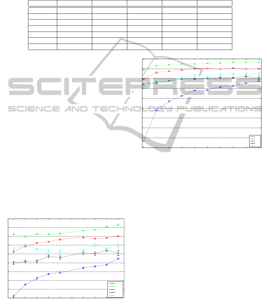
Table 1: Classification accuracy (± standard error) on unattributed graph datasets. OUR denotes the proposed model. SA
QJSD and QJSU denote the Quantum Jensen-Shannon kernel in the aligned (Torsello et al., 2014) and unaligned (Bai et al.,
2013) version, WL is the Weisfeiler-Lehman kernel (Shervashidze et al., 2011), GR denotes the graphlet kernel computed
using all graphlets of size 3 (Shervashidze et al., 2009), SP is the shortest-path kernel (Borgwardt and peter Kriegel, 2005),
and RW is the random walk kernel (Kashima et al., 2003). For each classification method and dataset, the best performance
is highlighted in bold.
Datasets PPI PTC COIL5 Reeb MUTAG
OUR 79.60 ± 0.86 76.80 ± 1.52 86.41 ± 0.38 67.36 ± 1.52 87.74 ± 0.47
QJSD 68.86 ± 1.00 55.78 ± 0.38 69.83 ± 0.22 35.03 ± 0.26 81.00 ± 0.51
SA QJSD 68.56 ± 0.87 57.07 ± 0.34 69.90 ± 0.22 35.78 ± 0.42 82.11 ± 0.30
WL 79.40 ± 0.83 56.86 ± 0.37 29.08 ± 0.57 50.73 ± 0.39 77.94 ± 0.46
GR 51.06 ± 1.00 55.70 ± 0.18 66.49 ± 0.25 22.90 ± 0.36 81.05 ± 0.41
SP 63.25 ± 0.97 56.32 ± 0.28 69.28 ± 0.42 55.85 ± 0.37 83.36 ± 0.52
RW 49.93 ± 0.83 55.78 ± 0.07 11.83 ± 0.17 15.98 ± 0.42 79.61 ± 0.64
the datasets (both training and test set) and apply our
classification method to it.
Fig. 2 shows the average classification accuracy
(± standard error) on all the datasets as we vary the
number of eigenvectors used. As you can see, ev-
ery dataset behave differently based on the number of
eigenvectors involved. In particular, for the COIL5
dataset, the use of more eigenvectors yields worst re-
sults, which means that the eigenvectors associated to
the smaller non-zero eigenvalues of the spectra, mod-
els the classes better, while the subsequent ones just
add noise to our representation. In the contrary, the
Mutag dataset benefits from increasing the number
of eigenvectors (and eigenvalues) involved in the cre-
ation of the class model.
Fig.3 shows the average classification accuracy (±
standard error) on all the datasets as we vary the per-
centage of sub-sampling applied to each graph of each
dataset. In particular, the first accuracy measure cor-
responds to the application of our model on the spec-
tral decomposition of the graphs where only 10% of
the nodes were preserved. All the datasets (except
for Mutag and PPI datasets) reach worse levels of ac-
Graph sampling percentage
Average accuracy
Accuracy variations after graph sub-sampling
0.1 0.2 0.3 0.4 0.5 0.6 0.7 0.8 0.9 1
0.45
0.5
0.55
0.6
0.65
0.7
0.75
0.8
0.85
0.9
COIL5
Mutag
Reeb
PTC
PPI
Figure 3: Average classification accuracy (with the inter-
val segment representing the ± standard error) on all the
datasets as we vary the percentage of sub-sampling applied
to each graph of each dataset.
Training set percentage
Average accuracy
Accuracy variations over training set dimension
0.1 0.2 0.3 0.4 0.5 0.6 0.7 0.8 0.9 1
0
0.1
0.2
0.3
0.4
0.5
0.6
0.7
0.8
0.9
COIL5
Mutag
Reeb
PTC
PPI
Figure 4: Average classification accuracy (with the inter-
val segment representing the ± standard error) on all the
datasets as we vary the percentage of graph of the training
set used to build the model.
curacy with a lower number of nodes, meaning that
the structural information given by each node of the
model is useful for classification purpose. Conversely,
the other datasets are more robust to sub-sampling.
Table 1 shows the average classification accuracy
(± standard error) of the different kernels and of our
method on the selected datasets. The proposed model
yields an increase of the performance with respect to
the confronted graph kernels on all the used datasets.
In particular, we obtained similar results with respect
to the Weisfeiler-Lehman graph kernel on the PPI
dataset. This is probably due to the use of the node
labels in order to mitigate the localization problem
and thus improving node localization in the evalua-
tion process. Even though our model does not exploit
node attributes, we were able to outperform all the
kernels on all the other datasets.
ICPRAM2015-InternationalConferenceonPatternRecognitionApplicationsandMethods
318

4 CONCLUSION
In this paper we have introduced a novel model
of structural representation based on a spectral de-
scription of graphs which lifts the one-to-one node-
correspondence assumption and is strongly rooted in
a statistical learning framework. We showed how the
defined separate models for eigenvalues and eigen-
vectors could be used within a statistical framework
to address the graphs classification task. We tested the
defined method against a number of alternative graph
kernels and we showed its effectiveness in a number
of structural classification tasks.
REFERENCES
Aubry, M., Schlickewei, U., and Cremers, D. (2011). The
wave kernel signature: A quantum mechanical ap-
proach to shape analysis. In Computer Vision Work-
shops (ICCV Workshops), 2011 IEEE International
Conference on, pages 1626–1633.
Bai, L., Hancock, E., Torsello, A., and Rossi, L. (2013).
A quantum jensen-shannon graph kernel using the
continuous-time quantum walk. In Kropatsch, W.,
Artner, N., Haxhimusa, Y., and Jiang, X., editors,
Graph-Based Representations in Pattern Recognition,
Lecture Notes in Computer Science, pages 121–131.
Springer Berlin Heidelberg.
Biasotti, S., Marini, S., Mortara, M., Patan, G., Spagnuolo,
M., and Falcidieno, B. (2003). 3d shape matching
through topological structures. In Nystrm, I., San-
niti di Baja, G., and Svensson, S., editors, Discrete
Geometry for Computer Imagery, volume 2886 of
Lecture Notes in Computer Science, pages 194–203.
Springer Berlin Heidelberg.
Bonev, B., Escolano, F., Lozano, M., Suau, P., Cazorla, M.,
and Aguilar, W. (2007). Constellations and the un-
supervised learning of graphs. In Escolano, F. and
Vento, M., editors, Graph-Based Representations in
Pattern Recognition, volume 4538 of Lecture Notes
in Computer Science, pages 340–350. Springer Berlin
Heidelberg.
Borgwardt, K. M. and peter Kriegel, H. (2005). Shortest-
path kernels on graphs. In In Proceedings of the 2005
International Conference on Data Mining, pages 74–
81.
Bunke, H., Foggia, P., Guidobaldi, C., and Vento, M.
(2003). Graph clustering using the weighted mini-
mum common supergraph. In Hancock, E. and Vento,
M., editors, Graph Based Representations in Pattern
Recognition, volume 2726 of Lecture Notes in Com-
puter Science, pages 235–246. Springer Berlin Hei-
delberg.
Estrada, F. and Jepson, A. (2009). Benchmarking im-
age segmentation algorithms. International journal of
computer vision, 85(2):167–181.
Friedman, N. and Koller, D. (2003). Being bayesian about
network structure. a bayesian approach to structure
discovery in bayesian networks. Machine Learning,
50(1-2):95–125.
Jensen, L. J., Kuhn, M., Stark, M., Chaffron, S., Creevey,
C., Muller, J., Doerks, T., Roth, E., Simonovic, M.,
Bork, P., and Mering, C. V. (2008). String 8 a global
view on proteins and their functional interactions in
630 organisms.
Kashima, H., Tsuda, K., and Inokuchi, A. (2003). Marginal-
ized kernels between labeled graphs. In Proceedings
of the Twentieth International Conference on Machine
Learning, pages 321–328. AAAI Press.
Li, G., Semerci, M., Yener, B., and Zaki, M. J. (2012). Ef-
fective graph classification based on topological and
label attributes. Stat. Anal. Data Min., pages 265–283.
Litman, R. and Bronstein, A. M. (2014). Learning spec-
tral descriptors for deformable shape correspondence.
IEEE Trans. Pattern Anal. Mach. Intell., 36(1):171–
180.
Luo, B., Wilson, R. C., and Hancock, E. R. (2006). A
spectral approach to learning structural variations in
graphs. Pattern Recognition, 39(6):1188 – 1198.
Nene, S. A., Nayar, S. K., and Murase, H. (1996). Columbia
Object Image Library (COIL-20). Technical report.
Shervashidze, N., Schweitzer, P., van Leeuwen, E. J.,
Mehlhorn, K., and Borgwardt, K. M. (2011).
Weisfeiler-lehman graph kernels. J. Mach. Learn. Res.
Shervashidze, N., Vishwanathan, S. V. N., Petri, T. H.,
Mehlhorn, K., and et al. (2009). Efficient graphlet ker-
nels for large graph comparison.
Silverman, B. W. (1986). Density Estimation for Statistics
and Data Analysis. Chapman & Hall, London.
Todorovic, S. and Ahuja, N. (2006). Extracting subimages
of an unknown category from a set of images. In
Computer Vision and Pattern Recognition, 2006 IEEE
Computer Society Conference on, volume 1, pages
927–934.
Torsello, A. (2008). An importance sampling approach to
learning structural representations of shape. In Com-
puter Vision and Pattern Recognition, 2008. CVPR
2008. IEEE Conference on, pages 1–7.
Torsello, A., Gasparetto, A., Rossi, L., and Hancock, E.
(2014). Transitive State Alignment for the Quantum
Jensen-Shannon Kernel.
Torsello, A. and Hancock, E. (2006). Learning shape-
classes using a mixture of tree-unions. Pattern Anal-
ysis and Machine Intelligence, IEEE Transactions on,
28(6):954–967.
Torsello, A. and Rossi, L. (2011). Supervised learning of
graph structure. In Pelillo, M. and Hancock, E. R.,
editors, SIMBAD, volume 7005 of Lecture Notes in
Computer Science, pages 117–132. Springer.
White, D. and Wilson, R. (2007). Spectral generative mod-
els for graphs. In Image Analysis and Processing,
2007. ICIAP 2007. 14th International Conference on,
pages 35–42.
ANon-parametricSpectralModelforGraphClassification
319
