Model Guided Sampling Optimization for Low-dimensional Problems
Lukáš Bajer
1,2
and Martin Hole
ˇ
na
1
1
Institute of Computer Science, Academy of Sciences of the Czech Republic,
Pod Vodárenskou vˇeží 2, Prague, Czech Republic
2
Faculty of Mathematics and Physics, Charles University in Prague, Malostranské nám. 25, Prague, Czech Republic
Keywords:
black-box Optimization, Gaussian Process, Surrogate Modelling, EGO.
Abstract:
Optimization of very expensive black-box functions requires utilization of maximum information gathered by
the process of optimization. Model Guided Sampling Optimization (MGSO) forms a more robust alternative
to Jones’ Gaussian-process-based EGO algorithm. Instead of EGO’s maximizing expected improvement,
the MGSO uses sampling the probability of improvement which is shown to be helpful against trapping in
local minima. Further, the MGSO can reach close-to-optimum solutions faster than standard optimization
algorithms on low dimensional or smooth problems.
1 INTRODUCTION
Optimization of expensive empirical functions forms
an important topic in many engineering or natural-
sciences areas. For such functions, it is often impos-
sible to obtain any derivatives or information about
smoothness; moreover, there is no mathematical ex-
pression nor an algorithm to evaluate. Instead, some
simulation or experiment has to be performed, and the
value obtained through a simulation or experiment is
the value of the objective function being considered.
Such functions are also called black-box functions.
They are usually very expensive to evaluate; one eval-
uation may cost a lot of time and money to process.
Because of the absence of derivatives, standard
continuous first- or second-order derivative optimiza-
tion methods cannot be used. In addition, the func-
tions of this kind are usually characterized by a high
number of local optima where simple algorithms can
be trapped easily. Therefore, different derivative-free
optimization methods (often called meta-heuristics)
have been proposed. Even though these methods are
rather slow and sometimes also computationally in-
tensive, the cost of the empirical function evaluations
is always much higher and the cost of these evalu-
ations dominates the computational cost of the opti-
mization algorithm. For this reason, it is crucial to
decrease the number of function evaluations as much
as possible.
Evolutionary algorithms constitute a broad family
of meta-heuristics that are frequently used for black-
box optimization. Furthermore, some additional al-
gorithms and techniques have been designed to min-
imize the number of objective function evaluations.
All of the three following approaches use a model (of
a different type in each case), which is built and up-
dated within the optimization process.
Estimation of distribution algorithms (EDAs)
(Larrañaga and Lozano, 2002) represent one such
approach: EDAs iteratively estimate the distribution
of selected solutions (usually solutions with fitness
above some threshold) and sample this distribution
forming a new set of solutions for the next iteration.
Surrogate modelling is the technique of learning
and usage of a regression model of the objective func-
tion (Jin, 2005). The model (called surrogate model
in this context) is then used to evaluate some of the
candidate solutions instead of the original costly ob-
jective function.
Our method, Model Guided Sampling Optimiza-
tion (MGSO), takes inspiration from both these ap-
proaches. It uses a regression model of the objective
function, which also provides an error estimate. How-
ever, instead of replacing the objective function with
this model, it combines its prediction and the error es-
timate to get a probability of reaching a better solution
in a given point. Similarly to EDAs, the MGSO then
samples this pseudo-distribution
1
, in order to obtain
1
a function proportional to a probability distribution, it’s
value is given by the probability of improvement
451
Bajer L. and Hole
ˇ
na M..
Model Guided Sampling Optimization for Low-dimensional Problems.
DOI: 10.5220/0005222404510456
In Proceedings of the International Conference on Agents and Artificial Intelligence (ICAART-2015), pages 451-456
ISBN: 978-989-758-074-1
Copyright
c
 2015 SCITEPRESS (Science and Technology Publications, Lda.)

the next set of solution candidates.
The MGSO is also similar to Jones’ Efficient
Global Optimization (EGO) (Jones et al., 1998).
Like EGO, the MGSO uses a Gaussian process (GP,
see (Rasmussen and Williams, 2006) for reference),
which provides a guide where to sample new candi-
date solutions in order to explore new areas and ex-
ploit promising parts of the objective-function land-
scape. Where EGO selects a single or very few solu-
tions maximizing a chosen criterion – Expected Im-
provement (EI) or Probability of Improvement (PoI)
– the MGSO samples the latter criterion. At the same
time, the GP serves for the MGSO as a surrogate
model of the objective function for a small proportion
of the solutions.
This paper further develops the MGSO algorithm
introduced in (Bajer et al., 2013). It brings several im-
provements (new optimization procedures and more
general covariance function) and performance com-
parison to EGO. The following section introduces
methods used in the MGSO, Section 3 describes the
MGSO algorithm, and Section 4 comprises some
experimental results on several functions from the
BBOB testing set (Hansen et al., 2009).
2 GAUSSIAN PROCESSES
Gaussian process is a probabilistic model based on
Gaussian distributions. This type of model was cho-
sen because it predicts the function value in a new
point in the form of univariate Gaussian distribution:
the mean and the standard deviation of the function
value are provided. Through the predicted mean, the
GP can serve as a surrogate model, and the standard
deviation is an estimate of the prediction uncertainty
in a new point.
The GP is specified by mean and covariance func-
tions and a relatively small number of covariance
function’s hyper-parameters. The hyper-parameters
are usually fitted by the maximum-likelihood method.
Let X
N
= {x
i
| x
i
∈ R
D
}
N
i=1
be a set of N training
D-dimensional data points with known dependent-
variable values y
N
= {y
i
}
N
i=1
and f (x) be an unknown
function being modelled for which f (x
i
) = y
i
for all
i ∈ {1,...,N}. The GP model imposes a probabilis-
tic model on the data: the vector of known func-
tion values y
N
is considered to be a sample of a N-
dimensional multivariate Gaussian distribution with
the value of the probability density p(y
N
|X
N
). If we
take into consideration a new data point (x
N+1
,y
N+1
),
the value of the probability density in the new point is
p(y
N+1
|X
N+1
) =
exp(−
1
2
y
>
N+1
C
−1
N+1
y
N+1
)
p
(2π)
N+1
det(C
N+1
)
(1)
where C
N+1
is the covariance matrix of the Gaussian
distribution (for which mean is usually set to constant
zero) and y
N+1
= (y
1
,...,y
N
,y
N+1
) (see (Buche et al.,
2005) for details). This covariance can be written as
C
N+1
=

C
N
k
k
>
κ

(2)
where C
N
is the covariance of the Gaussian distribu-
tion given the N training data points, k is the vector of
covariances between the new point and training data,
and κ is the variance of the new point itself.
Predictions. Predictions in Gaussian processes are
made using Bayesian inference. Since the inverse
C
−1
N+1
of the extended covariance matrix can be ex-
pressed using the inverse of the training covariance
C
−1
N
, and y
N
is known, the density of the distribution
in a new point simplifies to a univariate Gaussian with
the density
p(y
N+1
|X
N+1
,y
N
) ∝ exp −
1
2
(y
N+1
− ˆy
N+1
)
2
s
2
y
N+1
!
(3)
with the mean and variance given by
ˆy
N+1
= k
>
C
−1
N
y
N
, (4)
s
2
y
N+1
= κ − k
>
C
−1
N
k. (5)
Further details can be found in (Buche et al., 2005).
Covariance Functions. The covariance C
N
plays a
crucial role in these equations. It is defined by the
covariance-function matrix K and signal noise σ as
C
N
= K
N
+ σI
N
(6)
where I
N
is the identity matrix of order N. Gaus-
sian processes use parametrized covariance functions
K describing prior assumptions on the shape of the
modelled function. The covariance between the func-
tion values at two data points x
i
and x
j
is given by
K(x
i
,x
j
), which forms the (i, j)-th element of the
matrix K
N
. We used the most common squared-
exponential function
K(x
i
,x
j
) = θ exp

−
1
2`
2
(x
i
− x
j
)
>
(x
i
− x
j
)

, (7)
which is suitable when the modelled function is rather
smooth. The closer the points x
i
and x
j
are, the
closer the covariance function value is to 1 and the
stronger correlation between the function values f (x
i
)
and f (x
j
) is. The signal variance θ scales this correla-
tion, and the parameter ` is the characteristic length-
scale with which the distance of two considered data
points is compared. Our choice of the covariance
function was motivated by its simplicity and the pos-
sibility of finding the hyper-parameter values by the
maximum-likelihood method.
ICAART2015-InternationalConferenceonAgentsandArtificialIntelligence
452

3 MODEL GUIDED SAMPLING
OPTIMIZATION (MGSO)
The MGSO algorithm is based on a similar idea as
EGO. It heavily relies on Gaussian process modelling,
particularly on its regression capabilities and ability
to assess model uncertainty in any point of the input
space.
While most variants of EGO calculate new points
from the expected improvement (EI), The MGSO uti-
lizes the probability of improvement which is closer
to the basic concept of the MGSO: sampling a distri-
bution of promising solutions
2
.
This probability is taken as a function proportional
to a probability density and is sampled producing a
whole population of candidate solutions – individuals.
This is the main difference to EGO which takes only
very few individuals each iteration, usually the point
maximizing EI.
3.1 Sampling
The core step of the MGSO algorithm is the sampling
of the probability of improvement. This probability
is, for a chosen threshold T of the function value, di-
rectly given by the predicted mean
ˆ
f (x) = ˆy and the
standard deviation ˆs(x) = s
y
of the GP model
ˆ
f in any
point x of the input space
PoI
T
(x) = P(
ˆ
f (x) 5 T ) = Φ

T −
ˆ
f (x)
ˆs(x)

, (8)
which corresponds to the value of cumulative distri-
bution function (CDF) of the Gaussian with density
(3) for the value of threshold T . As a threshold T , val-
ues near the so-far optimum (or the global optimum if
known) are usually taken.
Even though all the variables come from Gaussian
distribution, PoI(x) is definitely not Gaussian-shaped
since it depends on the threshold T and the black-box
function being modelled f . A typical example of the
landscape of PoI(x) in two dimensions for the Rastri-
gin function is depicted in Fig. 1. The dependency on
the black-box function also causes the lack of analyt-
ical marginals or derivatives.
3.2 MGSO Procedure
The MGSO algorithm starts with an initial random
sample from the input space forming an initial pop-
ulation, which is evaluated with the black-box objec-
tive function (step (2) in Alg. 1). All the evaluated
solutions are saved to a database from where they are
used as a training set for the GP model.
2
some EGO variants use PoI, too (Jones, 2001)
−5 0 5
−5
0
5
0.1
0.2
0.3
0.4
0.5
0.6
0.7
0.8
0.9
Figure 1: Probability of improvement. Rastrigin function in
2D, the GP model is built using 40 data points.
Algorithm 1: MGSO (Model Guided Sampling Optimiza-
tion).
1: Input: f – black-box objective function
N – standard population size
r – the number of solutions for dataset restriction
2: S
0
= {(x
j
,y
j
)}
N
j=1
← generate N initial samples and
evaluate them by f : y
j
= f (x
j
)
3: while no stopping condition is met, for i = 1, 2, .. . do
4: M
i
← build a GP model and fit its hyper-parameters
according to the dataset S
i−1
5: {x
j
}
N
j=1
← sample the PoI
M
i
T
(x) forming N new
points, optionally with different targets T
6: x
min
← argmin
x
ˆ
f (x) – find the minimum of the GP
(by local cont. optimization) and replace the nearest
solution from {x
j
}
N
j=1
with it
7: {y
j
}
N
j=1
← f ({x
j
}
N
j=1
) {evaluate the population}
8: S
i
← S
i−1
∪ {(x
j
,y
j
)}
N
j=1
{augment the dataset}
9: (x
min
,y
min
) ← argmin
(x,y)∈S
i
y
{find the best solution in S
i
}
10: if any rescale condition is met then
11: restrict the dataset S
i
to the bounding-box [l
i
,u
i
]
of the r nearest solutions along the best solution
(x
min
,y
min
) and linearly transform S
i
to [−1,1]
D
12: end if
13: end while
14: Output: the best found solution (x
min
,y
min
)
The main cycle of the MGSO starts with fitting
the GP model’s (M
i
) hyper-parameters based on the
data from the current dataset S
i
(step (4)). Further, the
model’s PoI
M
i
T
is sampled (step (5)) and supplemented
with the GP model’s minimum (step (6)), forming up
to N new individuals {x
j
}
N
j=1
where N is a parameter
defining the standard population size. The algorithm
follows up with the evaluation of the new individuals
with the objective function (step (7)), extending the
dataset of already-measured samples (step (8)) and
finding the best so-far optimum (x
min
,y
min
) (step (9)).
Covariance Matrix Constraint. As every covari-
ance matrix, Gaussian process’ covariance matrix is
required to be positive semi-definite (PSD). This con-
straint is checked during sampling, and candidate so-
ModelGuidedSamplingOptimizationforLow-dimensionalProblems
453

lutions leading to close-to-indefinite matrix are re-
jected. Although it could cause smaller population-
size in some iterations, it is an important step: other-
wise, Gaussian process training and fitting becomes
numerically very unstable. If such rejections arise,
other two thresholds T for calculating PoI are tested
and population with the greatest cardinality is taken.
These rejections occur when the GP model is suffi-
ciently trained and sampled solutions become close
to the model’s predicted values.
Model Minimum. New population is supple-
mented with the minimum x
min
of the model’s pre-
dicted values found by continuous optimization
3
(step
(6), x
min
= argmin
x
ˆ
f (x)); more precisely, the nearest
sampled solution is replaced with this minimum (un-
less less than N solutions were sampled).
Input Space Restriction. In current implementa-
tion, MGSO requires bounds constraints x ∈ [l,u], l <
u ∈ R
D
to be defined on the input space, which is used
by the algorithm to internal linear scaling of the input
space to hypercube [−1, 1]
D
. As the algorithm pro-
ceeds, the input space can be restricted along the so-
far optimum to a smaller bounding box (steps (10)–
(12)) which is again linearly scaled to [−1, 1]
D
. The
size of the new box is defined as a bounding box of r
nearest samples from the current so-far optimum x
min
;
enlarged by 10% at the boundaries. For the parameter
r = 15 · D was used as a rule of thumb.
This process not only speeds up model fitting
and prediction (due to the smaller number of train-
ing data), but focuses the optimization along the best
found solution and broaden small regions of non-zero
PoI.
Several criteria are defined to launch such input
space restriction, from which the most important is
occurrence of numerous rejections in sampling due
to close-to-indefinite covariance matrix. If the result-
ing new bounding box from the restriction is close to
the previous box (the coordinates are not smaller than
[−0.8,0.8]
D
), the input space restriction is not per-
formed.
3.3 Gaussian Processes Implementation
Our Matlab implementation of the MGSO makes use
of Gaussian Process Regression and Classification
Toolbox (GPML Matlab code) – a toolbox accompa-
nying Rasmussen’s and Williams’ monograph (Ras-
mussen and Williams, 2006). In the current version of
3
Matlab’s fminsearch was used
the MGSO, Rasmussen’s optimization and model fit-
ting procedure minimize was replaced with fmincon
from Matlab Optimization toolbox and with Hansen’s
Covariance Matrix Adaptation (CMA-ES) (Hansen
and Ostermeier, 2001). These functions are used for
the minimization of GP’s negative log-likelihood in
model’s hyper-parameters fitting. Here, fmincon is
generally faster, but CMA-ES is more robust and does
not need a valid initial point.
The next improvement lies in the employment
of the diagonal-matrix characteristic length-scale pa-
rameter in the squared exponential covariance func-
tion, sometimes also called covariance function with
automatic relevance determination (ARD)
K
ARD
(x
i
,x
j
) =
θ exp

−
1
2
(x
i
− x
j
)
>
diag(
~
`)(x
i
− x
j
)

. (9)
The length-scale parameter ` in (7) changes to diag(
~
`)
– a matrix with diagonal elements formed by the ele-
ments of the vector
~
` ∈ R
D
. The application of ARD
was not straightforward, because hyper-parameters
training tends to stuck in local optima. These cases
were indicated by an extreme difference between the
different scale-length parameter
~
` components which
resulted in poor regression capabilities. Therefore,
constraints on maximum difference between compo-
nents of
~
` were introduced
~
`
i
≤ 2.5 kmedian(
~
`) −
~
`
i
k.
4 EXPERIMENTAL RESULTS
This section comprises quantitative results from sev-
eral tests of the MGSO as well as brief discussion
of the usability of the algorithm. The current Mat-
lab implementation of the MGSO algorithm
4
has been
tested on three different benchmark functions from
the BBOB testing set (Hansen et al., 2009): sphere,
Rosenbrock and Rastrigin function in three different
dimensionalities: 2D, 5D and 10D. For these cases,
comparison with CMA-ES – current state of the art
black-box optimization algorithm – and Tomlab’s im-
plementation of EGO
5
is provided.
The computational times are not quantified, but
whereas CMA-ES performs in orders of tens of sec-
onds, the running times of the MGSO and EGO
reaches up to several hours. We consider this draw-
back acceptable since the primary use of the MGSO is
4
the source is available at http://github.com/charypar/
gpeda
5
http://tomopt.com/tomlab/products/cgo/solvers/ego.php
ICAART2015-InternationalConferenceonAgentsandArtificialIntelligence
454

Sphere, 2D
Distance to optimum f
Δ
(log-scale 10
y
)
0 100 200 300 400 500
-10
-8
-6
-4
-2
0
2
4
Rosenbrock, 2D
Original evaluations
0 100 200 300 400 500
-10
-8
-6
-4
-2
0
2
4
Rastrigin, 2D
0 100 200 300 400 500
-8
-6
-4
-2
0
2
4
MGSO (isotrop.)
MGSO (ARD)
EGO (Tomlab)
CMA-ES
Sphere, 5D
Distance to optimum f
Δ
(log-scale 10
y
)
0 500 1000
-7
-6
-5
-4
-3
-2
-1
0
1
2
3
4
Rosenbrock, 5D
Original evaluations
0 500 1000
-7
-6
-5
-4
-3
-2
-1
0
1
2
3
4
Rastrigin, 5D
0 500 1000
0
0.5
1
1.5
2
2.5
MGSO (isotrop.)
MGSO (ARD)
EGO (Tomlab)
CMA-ES
Sphere, 10D
Distance to optimum f
Δ
(log-scale 10
y
)
0 500 1000 1500 2000 2500
-8
-7
-6
-5
-4
-3
-2
-1
0
1
2
3
Rosenbrock, 10D
Original evaluations
0 500 1000 1500 2000 2500
-1
0
1
2
3
4
5
Rastrigin, 10D
0 500 1000 1500 2000 2500
0
0.5
1
1.5
2
2.5
3
MGSO (isotrop.)
MGSO (ARD)
EGO (Tomlab)
CMA-ES
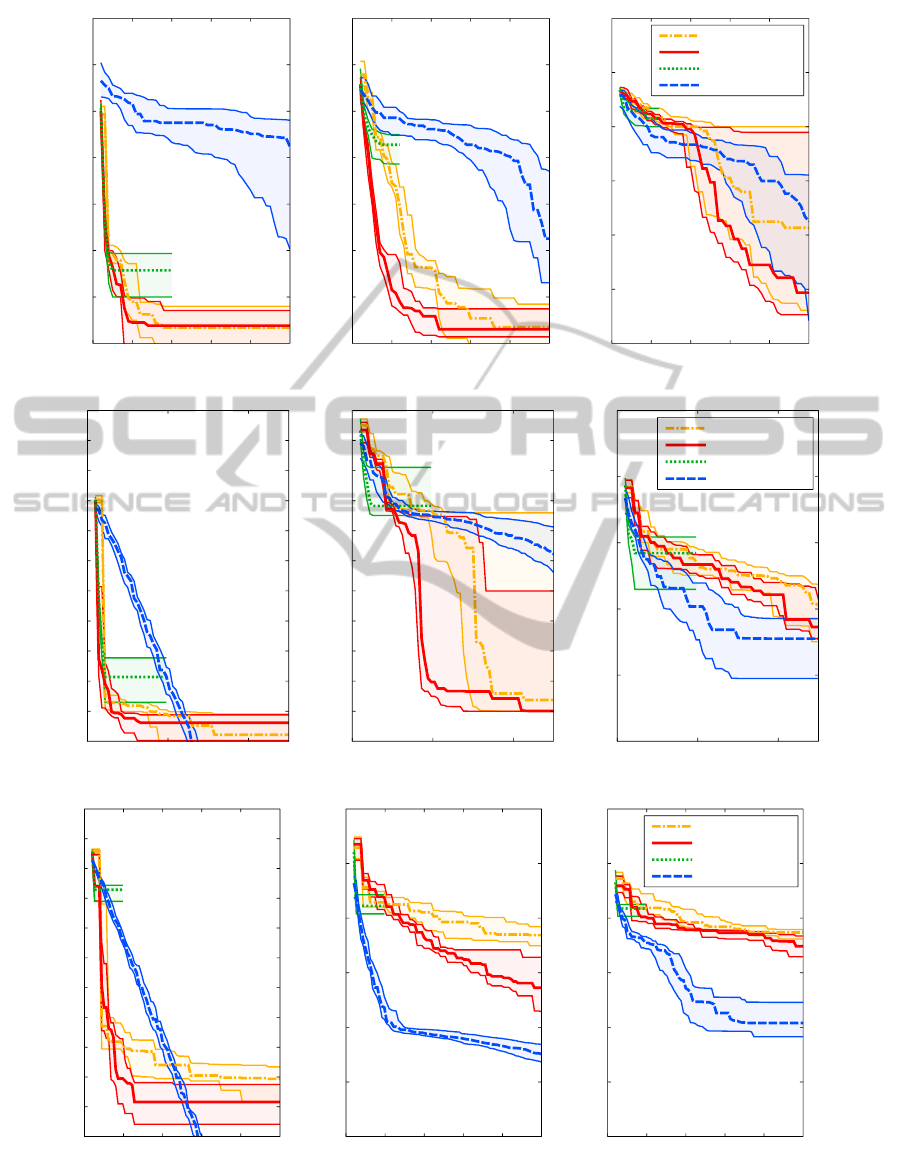
Figure 2: Medians, and the first and third quartiles of the distances from the best individual to optimum ( f
∆
= f
best
− f
OPT
)
with respect to the number of objective function evaluations for three benchmark functions. Quartiles are computed out of 15
trials with different initial settings (instances 1–5 and 31–40 in the BBOB framework).
ModelGuidedSamplingOptimizationforLow-dimensionalProblems
455

expensive black box optimization where a single eval-
uation of the objective function can easily take many
hours or even days and/or cost a considerable amount
of money (Hole
ˇ
na et al., 2008).
In the case of two-dimensional problems, the
MGSO performs far better than CMA-ES on
quadratic sphere and Rosenbrock function. The re-
sults on Rastrigin function are comparable, although
with greater variance (see Fig. 2: the descent of the
medians is slightly slower within the first 200 func-
tion evaluations, but faster thereafter). The Tomlab’s
implementation of EGO performs almost equally well
as the MGSO on sphere function, but on Rosenbrock
and Rastrigin, the convergence of EGO is extremely
slowed down after few iterations, which can be seen in
5D and 10D, too. The positive effect of ARD covari-
ance function can be seen quite clearly, especially on
Rosenbrock function. The difference between ARD
and non-ARD results are hardly to see on sphere func-
tion, probably because its symmetry means no im-
provement in ARD covariance employment.
The performance of the MGSO on five-
dimensional problems is similar to 2D cases.
The MGSO descends notably faster on non-rugged
sphere and Rosenbrock functions, especially if we
concentrate on depicted cases with a very low num-
ber of objective function evaluations (up to 250 · D
evaluations). The drawbacks of the MGSO is shown
on 5D Rastrigin function where it is outperformed
by CMA-ES, especially between ca. 200 and 1200
function evaluations.
Results of optimization in the case of ten-
dimensional problems show that the MGSO works
better than CMA-ES only on the most smooth sphere
function which is very easy to regress by Gaussian
process model. On more complicated benchmarks,
the MGSO is outperformed by CMA-ES.
The graphs on Fig. 2 show that the MGSO is
usually slightly slower than EGO in the very first
phases of the optimization, but EGO quickly stops its
progress and does not descent further. This is exactly
what can be expected from the MGSO in comparison
to EGO – sampling the PoI instead of searching for
the maximum can easily overcome situations where
EGO gets stuck in a local optimum.
5 CONCLUSIONS AND FUTURE
WORK
The MGSO, the optimization algorithm based on a
Gaussian process model and the sampling of the prob-
ability of improvement, is intended to be used in the
field of expensive black-box optimization. This pa-
per summarizes its properties and evaluates its perfor-
mance on several benchmark problems. Comparison
with Gaussian-process based EGO algorithm shows
that the MGSO is able to easily escape from local
optima. Further, it has been shown that the MGSO
can outperform state-of-the-art continuous black-box
optimization algorithm CMA-ES in low dimension-
alities or on very smooth functions. On the other
hand, CMA-ES performs better on rugged or high-
dimensional benchmarks.
ACKNOWLEDGEMENTS
This work was supported by the Czech Science Foun-
dation (GA
ˇ
CR) grants P202/10/1333 and 13-17187S.
REFERENCES
Bajer, L., Hole
ˇ
na, M., and Charypar, V. (2013). Improv-
ing the model guided sampling optimization by model
search and slice sampling. In Vinar, T. e. a., editor,
ITAT 2013 – Workshops, Posters, and Tutorials, pages
86–91. CreateSpace Indp. Publ. Platform.
Buche, D., Schraudolph, N., and Koumoutsakos, P. (2005).
Accelerating evolutionary algorithms with gaussian
process fitness function models. IEEE Transactions
on Systems, Man, and Cybernetics, Part C: Applica-
tions and Reviews, 35(2):183–194.
Hansen, N., Finck, S., Ros, R., and Auger, A. (2009).
Real-parameter black-box optimization benchmark-
ing 2009: Noiseless functions definitions. Technical
Report RR-6829, INRIA. Updated February 2010.
Hansen, N. and Ostermeier, A. (2001). Completely deran-
domized self-adaptation in evolution strategies. Evo-
lutionary Computation, 9(2):159–195.
Hole
ˇ
na, M., Cukic, T., Rodemerck, U., and Linke, D.
(2008). Optimization of catalysts using specific, de-
scription based genetic algorithms. Journal of Chem-
ical Information and Modeling, 48:274–282.
Jin, Y. (2005). A comprehensive survey of fitness approxi-
mation in evolutionary computation. Soft Computing,
9(1):3–12.
Jones, D. R. (2001). A taxonomy of global optimiza-
tion methods based on response surfaces. Journal of
Global Optimization, 21(4):345–383.
Jones, D. R., Schonlau, M., and Welch, W. J. (1998).
Efficient global optimization of expensive black-
box functions. Journal of Global Optimization,
13(4):455–492.
Larrañaga, P. and Lozano, J. A. (2002). Estimation of distri-
bution algorithms: A new tool for evolutionary com-
putation. Kluwer.
Rasmussen, C. E. and Williams, C. K. I. (2006). Gaussian
Processes for Machine Learning. Adaptative compu-
tation and machine learning series. MIT Press.
ICAART2015-InternationalConferenceonAgentsandArtificialIntelligence
456