Volumetric Quasi-conformal Mappings
Quasi-conformal Mappings for Volume Deformation with Applications to
Geometric Modeling
Alexander Naitsat
1
, Emil Saucan
1,2
and Yehoshua Y. Zeevi
3
1
Department of Mathematics, Technion, Haifa, Israel
2
School of Mathematical Sciences, Dalian University of Technology, Dalian, China
3
Electrical Engineering Department, Technion, Haifa, Israel
Keywords:
Quasi-conformal Maps, Volume Parameterization, Volumetric Meshes, Geometric Computing, Computer
Graphics.
Abstract:
Due to intrinsic differences between surfaces and higher dimensional objects, some important results regarding
surfaces can not be extended to volumetric domains. Most significantly, there exist no conformal volumetric
maps apart from M
¨
obius transformations. Although it is sometime stated explicitly, it is often overlooked that
existing methods of volume parameterization produce only quasi-conformal maps, which may be “far from
conformality”. We therefore introduce methods for assessing the extent of the local and global volumetric
deformation by means of the amount of conformal distortion produced. To this end we first illustrate basic
three-dimensional quasi-conformal deformations that are produced by parameterization techniques, and high-
light theoretical issues associated with spatial quasi-conformal mappings, and the relation that exists between
the geometry of the domain and conformal distortion.
1 INTRODUCTION
A conformal mapping, f : R
n
→ R
n
, is a 1:1 function
that preserves angles between intersecting curves.
Conformal maps are desirable in digital geometry
processing and computer graphics, since they do not
exhibit shear and, therefore preserve different vertex
properties as well as the qualities of the mesh itself.
From a mathematical viewpoint, conformal map-
ping of a domain D ⊂ R
n
is a smooth bijective func-
tion, which at any point x ∈ D equally scales the space
in every direction. This can be stated formally as
∀h ∈ R
n
: kd f
x
· hk = kd f
x
k · khk, (1)
where d f
x
denotes Jacobian matrix at point x.
The geometrical interpretation of (1) is that f
transforms an infinitely small sphere to a sphere.
There is a wide range of applications in computer
science and engineering for conformal parameteriza-
tion and deformation of a surface. However, by a
classical theorem of Liouville every conformal map-
ping of a domain in R
n
,n ≥ 3, is restricted to be a
M
¨
obius transformation, i.e. a composition of transla-
tions, uniform scaling, linear isometry and inversion
in a sphere. Therefore, most of the real-world ap-
plication can not produce conformal transformations
of volumetric data. Instead the transformation yields
the so called “quasi-conformal” mappings, which are
close, in some sense to satisfying conformality. Such
mappings can be understood intuitively as functions
that approximately preserve angles.
One of the methods in computer graphics used to
assess the degree of conformality of a 2D map f , is to
consider the ratio of singular values in the domain D
(Ahlfors, 2006),
max
x∈D
|σ
1
(x)|
|σ
n
(x)|
, (2)
where σ
1
(x) and σ
n
(x) are the maximal and minimal
singular values of d f
x
, respectively.
However, this approach is not accurate for dimen-
sions greater than 2, since it examines the behaviour
of f only in two directions.
In this paper we examine the problem of measur-
ing the conformal distortion, produced by a 3D trans-
formation. We also address issues related to the re-
lation between the geometry of the volume and the
minimal possible conformal distortion. Our approach
is based on the theory of quasi-conformal homeomor-
46
Naitsat A., Saucan E. and Zeevi Y..
Volumetric Quasi-conformal Mappings - Quasi-conformal Mappings for Volume Deformation with Applications to Geometric Modeling.
DOI: 10.5220/0005298900460057
In Proceedings of the 10th International Conference on Computer Graphics Theory and Applications (GRAPP-2015), pages 46-57
ISBN: 978-989-758-087-1
Copyright
c
 2015 SCITEPRESS (Science and Technology Publications, Lda.)

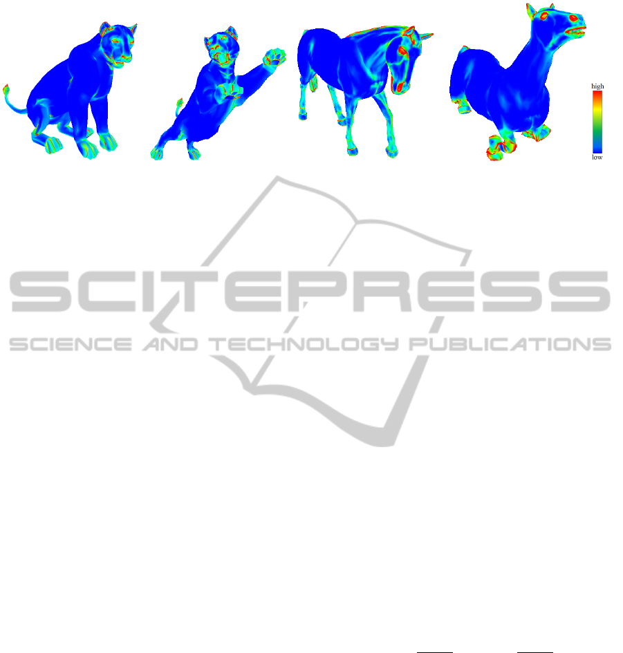
(a)
R
S
H
2
dA = 3265
R
S
H dA = 25.25
(b)
R
S
H
2
dA = 3124
R
S
H dA = 25.21
(c)
R
S
H
2
dA = 2267
R
S
H dA = 28.2
(d)
R
S
H
2
dA = 2751
R
S
H dA = 31
Figure 1: Diagram of mean curvature distribution for deformations of polygonal models.
Figures 1(a),1(b) represent domain and image of nearly isometric deformation that decreases W and
R
S
H by 4.3% and 0.1%,
respectively. Figures 1(c),1(d) represent domain and image of qc-deformation that increases W and
R
S
H by 21% and 10%,
respectively.
phism in R
n
. More precisely, we shall examine the
behaviour of f in a small neighbourhoods.
1.1 Conformal and Isometric Invariants
Given two homeomorphic domains D and D
0
in R
3
,
we wish to measure how close are these domains to
being conformally or isometrically equivalent. As the
first step in this estimation, we focus on boundaries of
the domains. We recall the following invariants of a
closed surface:
• Willmore energy of a surface S ⊂ R
3
, which is
conformal invariant (Willmore, 1993), defined by
W =
Z
S
H
2
dA − 4π + 4πg(S), (3)
where H represents the mean curvature and g(S)
is the genus of a surface. For a practical results
we assume that there are no changes in the genus.
Thus, we shall compute conformal invariant as
R
S
H
2
dA .
• Isometric invariant of a closed surface (Almgren
and Rivin, 1999) is
R
S
HdA.
Computation of invariants are shown in Figure 1
for triangular meshes, deformed by nearly-isometric
and quasi-conformal transformations, obtained by
discrete integration performed over the mesh vertices.
The area element dA was approximated by area of
barycentric cell around a vertex, mean curvature of
a vertex was computed via the half-tube formula (Lev
et al., 2007).
This method provides a naive approach for anal-
ysis of 3D domains, since it estimates only confor-
mal distortion produced on the boundary of volumet-
ric objects. To examine interior volumes we shall in-
troduce the basic theory of quasi-conformal mappings
in R
n
. Based on this theory we shall review the rela-
tion between the conformal distortion and the surface
of domains in subsection 3.6.
2 QUASI-CONFORMAL MAPS
2.1 Quasi-conformal Dilatations
Quasi-conformal mappings in R
n
can be studied by at
least two alternative approaches. The first approach
considers topological properties of a function along
the integrable curves. The other approach, which we
shall employ, examines the properties of a map in in-
finitely small neighbourhoods, where small spheres
are transformed into ellipsoids.
First we are going to restrict ourself to linear trans-
formations, for which we can define the following
quantities.
Definition 1. Let A : R
n
→ R
n
be linear 1:1 transfor-
mation. Define
K
I
(A) =
|detA|
l(A)
n
, K
O
(A) =
kAk
n
|detA|
, (4)
where
kAk = max
khk=1
kA · hk, l(A) = min
khk=1
kA · hk, (5)
and K
I
(A),K
O
(A) are called inner and outer dilata-
tions, respectively.
In the sequel we shall assume that all the functions
f : D → D
0
are diffeomorphisms, that is f is a smooth
bijective mapping with a smooth inverse. Hence, d f
x
is a full rank matrix, that maps a unit sphere S
n
onto
an ellipsoid E = d f
x
(S
n
). This leads itself to the fol-
lowing theorem:
VolumetricQuasi-conformalMappings-Quasi-conformalMappingsforVolumeDeformationwithApplicationsto
GeometricModeling
47

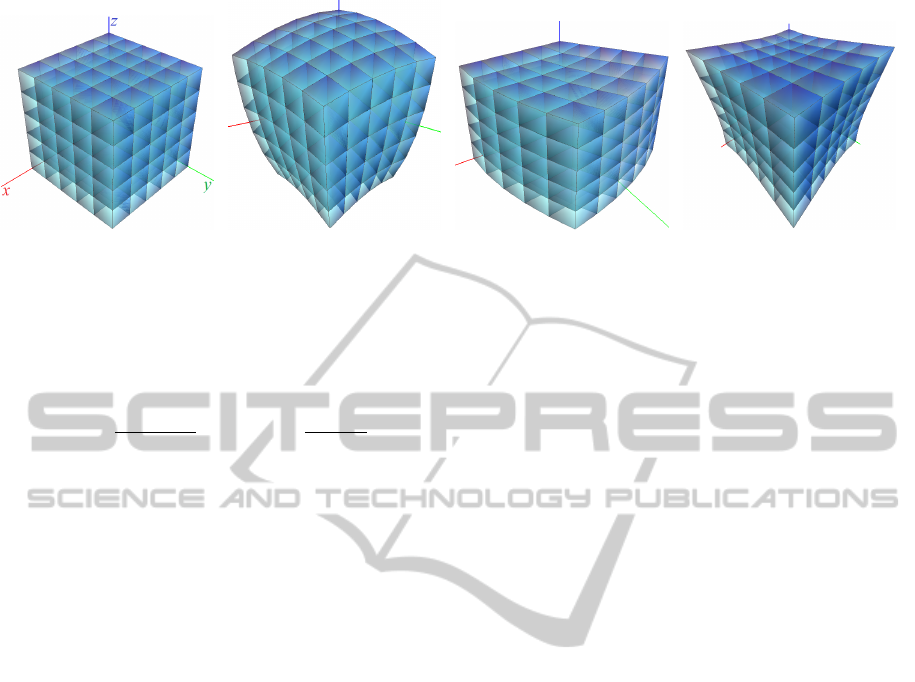
(a) Original (b) Cone, β/α = 1.4 (c) Folding, β/α = 1.4 (d) Radial, a = 1.7
Figure 2: Basic quasi-conformal mappings of a 5 × 5 × 5 grid.
Theorem 1. Let a
1
≥ a
2
≥ ....a
n
be semi axes of
E, then a
2
1
,...,a
2
n
are the eigenvalues of the matrix
d f
x
(d f
x
)
∗
and
K
I
(d f
x
) =
a
1
···a
n−1
a
n−1
n
, K
O
(d f
x
) =
a
n−1
1
a
2
···a
n
. (6)
Theorem 1 implies that a
1
,...,a
n
are the singular
values of d f
x
. In particular, a
1
= kd f
x
k is the longest
of the semi-axes of the ellipsoid, while a
n
= l(d f
x
) is
the shortest.
We define a quasi-conformal dilatation of f at a
point x as
K(x) = max
{
K
I
(d f
x
),K
O
(d f
x
)
}
, (7)
and the maximal quasi-conformal dilatation of f as
K( f ) = max
x∈D
K(x). (8)
We call f K-quasi-conformal, denoted by K-qc, if
K( f ) ≤ K for some constant number K.
The value of K( f ) can be considered as a measure
of departure from conformality of f . In particular,
K( f ) ≥ 1, and the equality holds if and only if f is
conformal.
2.2 Representation of Volumetric Data
Our first goal is to represent efficiently volumetric
data, and to demonstrate interesting qc-deformations.
We’ll then compute, numerically, changes in geomet-
rical properties of transformed domains. For these
tasks we shall employ simple volumetric meshes,
more precisely tetrahedal, and voxel meshes.
In addition to tetrahedral meshes produced from
triangular models of closed surfaces by “Tetgen” li-
brary (Si, 2009), we introduce voxel meshes. Voxel
meshes or voxelized volumes are regular hexahedral
meshes. Due to the regularity, voxel meshes are more
stable for numerical computations, although they are
much less flexible geometrically and generally repre-
sent only interior part of the volume.
Figure 4 depicts considerable differences in reg-
ularity and accuracy by which voxel and tetrahedral
meshes represent the same volume. As can be ob-
served, these differences become more pronounced
after a series of qc-deformations.
We propose an algorithm for generating a voxel
mesh from a polygonal mesh of a closed surface.
Our Algorithm 1 of Voxelization procedure is sim-
ilar to that of (Karabassi et al., 1999), with addi-
tional options for subdivision. This enables bet-
ter approximations of continues domains with rel-
atively low number of voxels. We run procedure
Voxelize(P,B, n
x
,n
y
,n
z
, d,k) to generate voxel mesh
M from polygonal mesh P of a closed surface, where
B equals to the bounding box of P. The resulting mesh
is denoted by
voxel(n
x
,n
y
,n
z
;d; k) . (9)
We often use such values of n
x
,n
y
,n
z
, that produce
cubic voxels. In such cases we denote the resulting
voxel-mesh by
cubic(n;d; k) , (10)
where n is the number of voxels along the longest axis
of the bounding box B. Figure 3 shows cross sec-
tions of the torus, represented by various volumetric
meshes, including both types of voxel meshes.
Testing whether a given point p is in interior of
the mesh P, denoted int(P), was done by traversing
ray from p and examining the number of intersection
points between the ray and the mesh. A point p is an
interior point of P if the number of intersection points
is even. For efficient and stable intersection test we
used ray traversing algorithm (Amanatides and Woo,
1987) and octree partition of the space (Perreault,
2007). Numerical issues may arise when a ray hits a
vertex of P. To cope with these issues, we assume that
two intersection points are equivalent if the distance
between them is below some predefined threshold.
GRAPP2015-InternationalConferenceonComputerGraphicsTheoryandApplications
48

Algorithm 1: Voxelize(P,B, n
x
,n
y
,n
z
,d, k).
Input:
P,B - polygonal mesh and bounding box
n
x
,n
y
,n
z
- number of voxels along the axes.
d - max depth of subdivisions
k - number of voxels in subdivision
M ← ∅
if d < 0 then
Quit
Devide B into n
x
× n
y
× n
z
grid
foreach voxel ϑ in the grid do
if All vertices of ϑ are inside P then
Add ϑ to M
else if At least one vertex of ϑ is inside P
then
B
ϑ
← Bounding box of ϑ
Voxelize(P,B
ϑ
, k,k,k, d − 1, k)
Output:
Partition of B ∩ int(P) into voxel mesh M
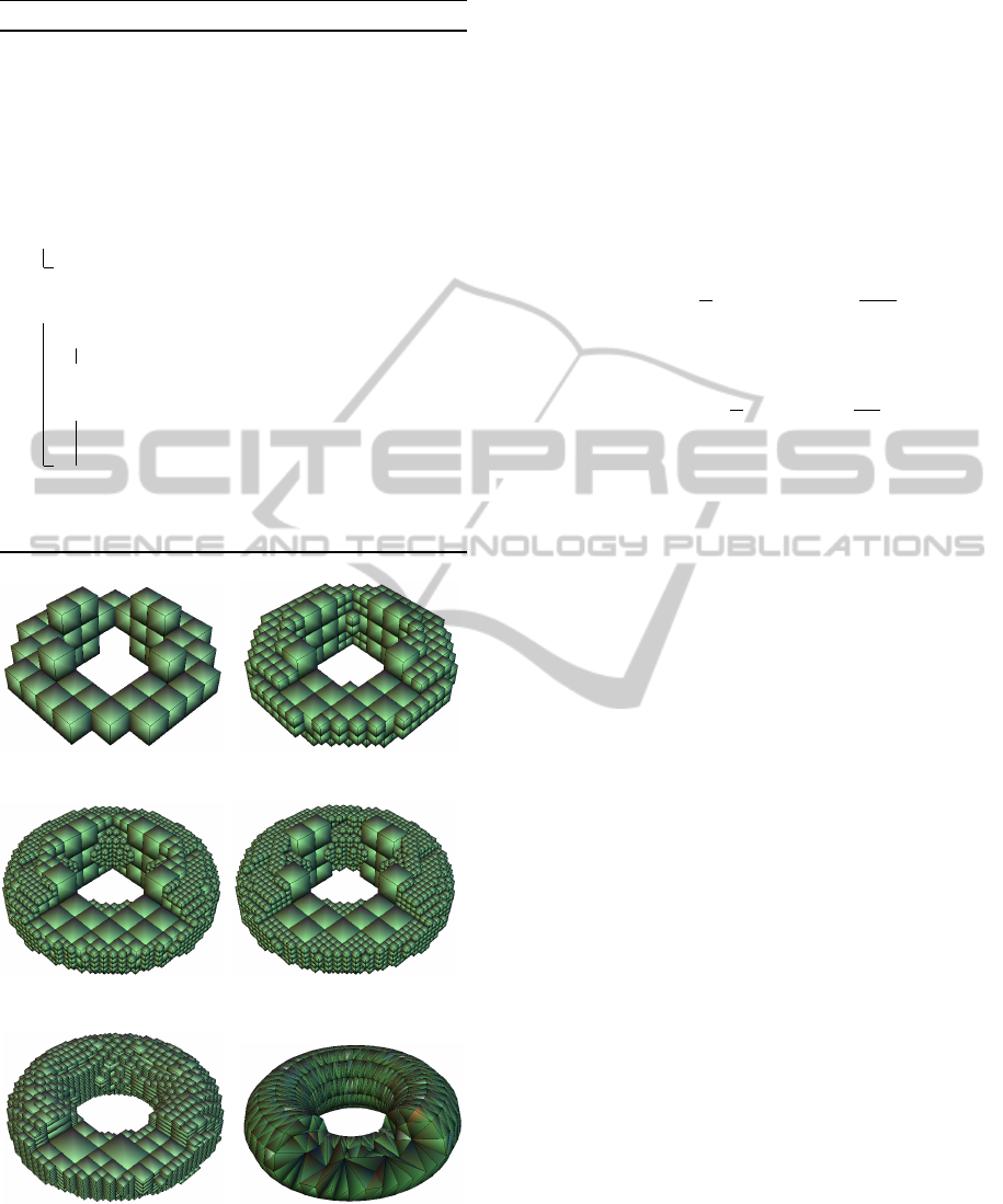
(a) cubic(10;0;2) (b) cubic(10;1;2)
(c) cubic(10;2;2) (d) cubic(10;1;4)
(e) voxel(6,8,8;2;2) (f) Tetrahedral mesh
Figure 3: Voxel meshes and the corresponding tetrahedral
mesh. All meshes were generated from the same polygonal
model of the torus.
2.3 Examples of 3D Quasi-conformal
Mappings
The simplest K-qc-map is an affine transformation.
The linear part of the transformation determines qc-
dilatation according to equation (4).
It’s easy to construct simple qc-maps by linear
transformations of cylindrical and spherical coordi-
nates. Setting constant ratio β/α ≥ 1 we can construct
a folding map in cylindrical coordinates by
F : (r,ϕ,z) 7→

r,
β
α
ϕ,z

, ϕ ∈

0,
2πα
β

, (11)
and cone map in spherical coordinates by
C(r, ϕ,θ) 7→

r, ϕ, θ
β
α

, θ ∈

0,
πα
β

. (12)
Computation of the dF yields (V
¨
ais
¨
al
¨
a, 1971,
pp. 49–50)
K
I
(F) = β/α, K
O
(F) = (β/α)
2
, (13)
Let ρ be an inversion in the unit sphere S
3
, which
is non-linear conformal map of R
3
\{0}. It’s easy to
extend ρ to a family of quasi-conformal maps ρ
a
for
a 6= 0 by
ρ
a
(x) = kxk
a−1
x for x 6= 0 (14)
In particular ρ = ρ
−1
(see Fig. 4).
Computation of d(ρ
a
)
x
shows that dilations of ra-
dial maps are domain-independent (V
¨
ais
¨
al
¨
a, 1971,
p. 49):
K(ρ
a
) =
(
max

|a|,a
2

|a| ≥ 1
max

a
−2
,|a|
−1

|a| ≤ 1
. (15)
We can construct more complicated qc-mappings
by looking for an analogue of conformal functions in
the plane. Zorich (Rickman, 1993) gave the exam-
ple of mapping Z : R
3
→ R
3
\{0}, which can be seen
as 3D extension of the complex exponential func-
tion. We shall present below qc-versions of the Zorich
mapping:
Set l > 0 and define infinite cylinders:
C
l
=
{
(x,y,z)
|
|x| ≤ l, |y| ≤ l
}
, (16)
˜
C
l
=

(x,y,z)
|
x
2
+ y
2
≤ l
2

,
and consider the following functions:
i. A radial stretching in planes R
3
× {z} of the
square with edge 2l into the circle of radius l
Z
1
: intC
l
→ int
˜
C
l
.
VolumetricQuasi-conformalMappings-Quasi-conformalMappingsforVolumeDeformationwithApplicationsto
GeometricModeling
49

(a) a=2.5 (b) a=1 original (c) a=-0.5 (d) a=-1 inversion on sphere
(e) a=-2 (f) a=2.5 (g) a=1 original (h) a=-1 inversion on sphere
Figure 4: Radial mappings of torus volume with different values of the parameter a. The torus is placed around origin and y
axis. Figures 4(a)-4(e) represent the volume by voxel mesh of the type cubic(10;2;2). Figures 4(f)-4(h) show cross sections
of the volume represented by tetrahedral mesh. Objects were rendered with transparency. Selected boundary vertex with its
1-ring were highlighted (relative sizes were not preserved).
ii. Quasi-conformal map of round cylinder into the
half-space
Z
2
: int
˜
C
l
→ H ,
defined by
Z
2
: (r, ϕ, z) 7→

e
z/l
,ϕ,
πr
2l

, (17)
where cylindrical and spherical coordinates, re-
spectively, are used.
We define Zorich map as
Z : intC
l
→ H, Z = Z
2
◦ Z
1
. (18)
This function can be applied on a model contained
in C
l
, thus we place models around the origin and set
l = a· r, where r is the radius of the bounding cylinder
and a ≥ 1 is a parameter that controls the distortion
level.
Figure 2 illustrates basic qc-deformations of the
cubic grid and Figure 5 shows some qc-mappings of
the polygonal model.
2.4 Quasi-conformal Parameterization
Consider a problem of volume parameterization into
the unit ball B
3
. We shall restrict ourself to the fol-
lowing domains:
Definition 2. Suppose D is a compact domain of R
3
containing a point p. Denote by
px the line segment
connecting p and x. The domain D is called star-
shaped at p, and p is called center of D if for any
x ∈ D px ⊂ D.
In particular, any convex domain is a star-shaped
domain, where any interior point can serve as the cen-
ter.
Without loss of generality, we shall focus on star-
shaped domains at 0 that satisfy the following geo-
metrical condition: for any ζ ∈ ∂D, the angle between
ζ0 and tangent plane at ζ is larger than or equal to
some constant α > 0. Any point x 6= 0 of such do-
main D has a unique representation
x = u(x)ζ(x) , (19)
where ζ(x) is an intersection point of ∂D and 0x, and
u(x) = kζ(x)k/kxk. Moreover, Caraman (Caraman,
1974, p. 408) had shown that for any a > 0 those do-
mains can be mapped quasi-conformally into B
3
by
f (x) =



u(x)
a
ζ(x)
kζ(x)k
x 6= 0
0 x = 0
. (20)
In fact any compact domain U, not necessarily
star-shaped, that satisfies the geometrical condition
GRAPP2015-InternationalConferenceonComputerGraphicsTheoryandApplications
50

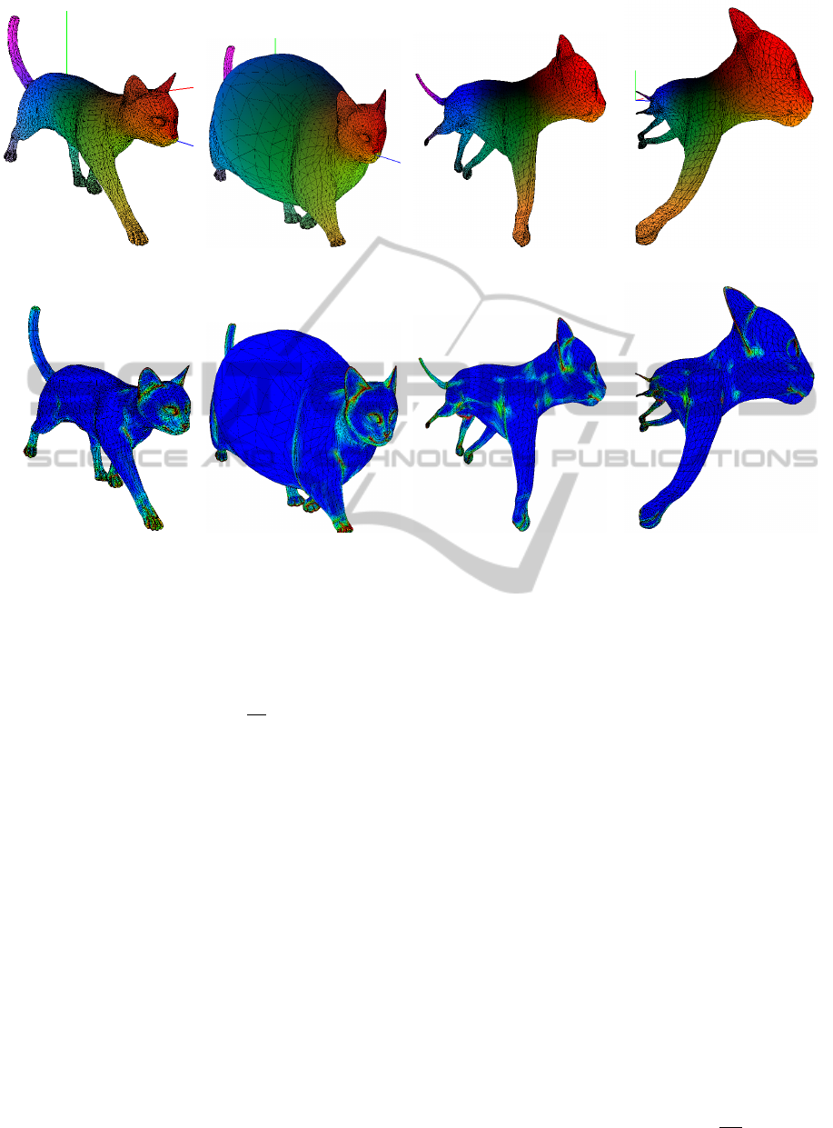
(a) Original model (b) Radial a = 0.4 (c) Zorich map a = 2 (d) Zorich map a = 1
(e) Original model (f) Radial a = 0.4 (g) Zorich map a = 2 (h) Zorich map a = 1
Figure 5: Quasi-conformal transformations of the polygonal mesh. 5(a)-5(d) are diagrams of spherical coordinates that
visualize transformations by domain coloring technique. R,G,B color values in these figures correspond to r,ϕ,θ coordinates
of the domain. 5(e)-5(h) are diagrams of mean curvature. Unit vectors are shown along the axes.
can be mapped quasi-conformally by (20) into sub-
domain of B
3
. We can consider U as a subdomain of
a star-shaped domain D and redefine ζ(x) as the far-
thest point from 0 of the set ∂D ∩ 0x .
Figure 8 show this qc-parameterization of tetrahe-
dral mesh into the unit ball for a = 1 .
3 COMPUTATION OF
QUASI-CONFORMAL
DILATATIONS
Our aim is to compute numerically qc-dilatations of
maps f : D → D
0
of discrete volumetric data, given
the following input:
i. Two polyhedral meshes of the domain M =
(V,E, F,C) and of its image M
0
= (V
0
,E
0
,F
0
,C
0
),
where V ,E,F and C are the vertex, edge, face and
cell sets of M, respectively, with the same notion
for M
0
.
ii. A transformation f defined on the set of mesh’s
vertices V . Depending on the context, we may
use f as the correspondence function between the
meshes.
f : (V,E,F,C) → (V
0
,E
0
,F
0
,C
0
).
The initial data can be defined explicitly by a con-
tinuous domain D and by a procedure that computes
f (x) for any x ∈ D. In this case we have a freedom to
generate appropriate polyhedral meshes to represent
the data.
The only necessary assumption about f is that it
should be a 1:1 function inside each polyhedral cell
c ∈ C. To find qc-dilatation of f at vertex v placed
at a position x ∈ R
3
, we need an estimation of the
Jacobian matrix d f
x
, more precisely we approximate
the following quantities: det(d f
x
), kd f
x
k and l(d f
x
).
3.1 Estimation of Jacobian Determinant
It is well known from elementary calculus that for a
diffeomorphism f : D → D
0
Z
D
0
dx
0
=
Z
D
J
f
(x)dx, J
f
(x) =
dx
0
dx
, (21)
VolumetricQuasi-conformalMappings-Quasi-conformalMappingsforVolumeDeformationwithApplicationsto
GeometricModeling
51

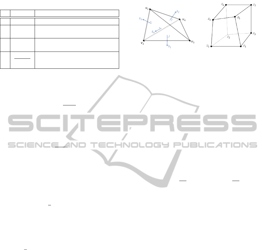
Table 1: Weights of the cell in Ring(v).
i w
i
(c) Description
1 1 Arithmetic average
2 m(c) Cell contribution is relative to its
volume
3 Ω(c, v) Solid angle of c measured from
the position of v
4
Ω(c,v)
m(c)
Combination of solid angle and
reverse volume weights
where J
f
(x) = det(d f
x
) will be referred as to “the Ja-
cobian”. Therefore an average value of the Jacobian
inside a cell c ∈C can be approximated by the volume
ratio
J
f
(c) =
m(c
0
)
m(c)
, (22)
where m(·) stands for a volume. We define a vertex
Jacobian, denoted by J
f
(v), as the weighted average
of the Jacobians in the neighboring cells
J
f
(v) =
∑
c∈Ring(v)
w(c)
m(c
0
)
m(c)
!
∑
c∈Ring(v)
w(c)
!
−1
,
(23)
where Ring(v) are the neighbouring cells of v and
w(c) is a chosen positive weight of the cell c (see Ta-
ble 1) .
The volume of a tetrahedron τ with the vertex po-
sitions x
0
,x
1
,x
2
,x
3
is
m(τ) =
1
6
det(x
10
,x
20
,x
30
) , (24)
where x
i j
= x
i
− x
j
.
For a hexahedron c with the vertex positions
x
0
,...,x
7
according to Figure 6(b) we can derive from
(Dukowicz, 1988) the following formula :
m(c) =
1
6
x
70
· (x
10
× x
35
+ x
40
× x
56
+ x
20
× x
63
).
(25)
3.2 Weights for Cells in 1-ring
Suppose we have a cell’s property P(c). We can es-
timate the corresponding property on a vertex P(v)
by a weighted average of P(c), taken over the neigh-
bouring cells c ∈ Ring(v). Table 1 summarizes some
methods to compute cell weights. In addition to the
common methods such as arithmetic and volume av-
eraging, we used the solid angle weights Ω(c, v) that
measure which part of the ε-ball around v is occupied
by c.
In a voxel mesh, each cell around a vertex v forms
the same solid angle, therefore solid angle weights for
voxels are equivalent to the arithmetic average.
(a) Tetrahedral cell (b) Hexahedron’s vertices
Figure 6: Cells of volumetric mesh.
Suppose τ is a tetrahedral cell shearing a vertex v
and σ is the face of τ against v. In geometry Ω(τ,v) is
a measure of how large τ appears to an observer look-
ing from v. Therefore Ω(τ,v) = Ω(σ,v), where the
last quantity can be computed from (van Oosterom A,
1983).
3.3 Basic Estimation of Singular Values
For a given vertex v and its edge e the length ratio
|e
0
|/|e| approximates kd f
x
· hk for a unit vector h in a
direction of edge e. Thus according to (5), our esti-
mations for the relevant singular values are
kd f
v
k = max
e∈Edge(v)
|e
0
|
|e|
, l (d f
v
) = min
e∈Edge(v)
|e
0
|
|e|
, (26)
where Edge(v) is the set of the neighbouring edges of
v.
The accuracy of this method depends on the va-
lence of v, i.e. the number of edges connected to v,
which is not always sufficiently large for a good ap-
proximation, especially for tetrahedal meshes, where
irregular direction of edges could cause significant
noise. (See Fig. 7(i) and 7(j).)
3.4 Estimation of Jacobian Matrix
We can estimate qc-dilatation of f at vertex v, placed
at a position x ∈ R
3
, based on estimation of the Jaco-
bian matrix d f
x
. First we estimate the average matrix
of d f inside a given cell c, denoted by d f
c
. Then we
define the vertex Jacobi matrix d f
v
as an average over
d f
c
in the neighbouring cells.
Let f
(1)
, f
(2)
, f
(3)
be the coordinate components
of the map f , where each one is a function from V to
R. We can express d f
c
as the matrix whose rows are
the average gradient vectors of f
(i)
.
Suppose r is a point inside tetrahedral cell τ,
which consists of vertices v
1
,v
2
,v
3
,v
4
. Let σ
j
be a
face against v
j
. Let s
j
be the vector along the nor-
mal of σ
j
, such that ks
j
k = Area(σ
j
) (see Fig. 6(a)),
GRAPP2015-InternationalConferenceonComputerGraphicsTheoryandApplications
52

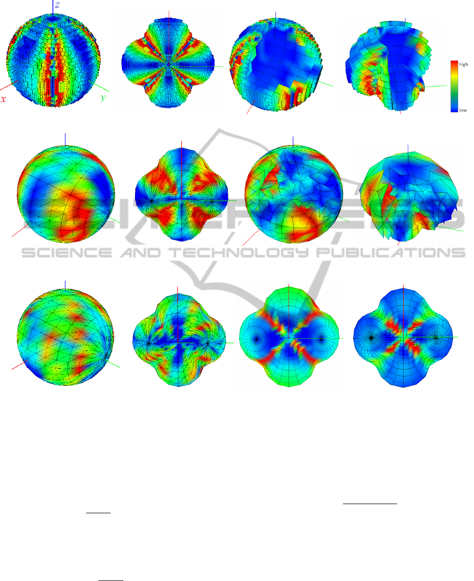
(a) K diagram of domain (b) K diagram of image (c) K diagram of domain (d) K diagram of image
(e) K diagram of domain (f) Kdiagram of image (g) K diagram of cross sec-
tion of the domain
(h) K diagram of cross sec-
tion of the image
(i) K diagram of domain (j) K diagram of image (k) Dihedral angles of image (l) Mean curvature of image
Figure 7: Zorich mapping with a = 1 of the ball placed at the origin. Dilatations were computed by default method except 7(i)
and 7(j), where the singular values were estimated by the length ratio method. Figures 7(a)-7(d) are voxel meshes, 7(e)-7(j)
are tetrahedral meshes, and 7(k), 7(l) are triangular meshes of volumes’ boundaries. Max K values, obtained for tetrahedral
and voxel meshes, are 4.6 and 4.55, respectively.
then for the piecewise linear extension of f we have
by (Wang et al., 2003)
f
(i)
(r) =
1
3m(τ)
4
∑
j=1
(r · s
j
) f
(i)
(v
j
). (27)
This implies that the gradient is constant inside τ,
hence our estimates give
∇ f
(i)
(τ) =
1
3m(τ)
4
∑
j=1
s
j
f
(i)
(v
j
); (28)
and
∇ f
(i)
(v) =
∑
c∈Ring(v)
∇ f
(i)
(c)ω(c), (29)
where ω(c) are normalized weights from the table 1
ω(c) =
w(c)
∑
η∈Ring(v)
w(η)
. (30)
We can extend above formulas for hexahedral mesh
without triangulation in a following way.
Suppose hexahedron c consists of vertices
v
1
,...,v
8
, and faces σ
1
,...,σ
6
(the enumeration is ar-
bitrary). Similarly to tetrahedron case, we define
s
j
to be a vector along the normal of σ
j
such that
ks
j
k = Area(σ
j
). Denote by
¯
σ
j
the face against σ
j
.
The face
¯
σ
j
contains 4 vertices against the face σ
j
,
we shall substitute them by single dummy vertex u
j
VolumetricQuasi-conformalMappings-Quasi-conformalMappingsforVolumeDeformationwithApplicationsto
GeometricModeling
53

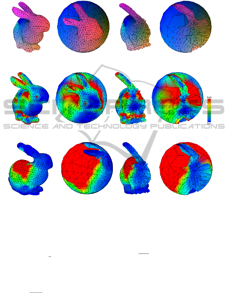
(a) Domain (b) Image (c) Cross section of the
domain
(d) Image of the cross section
(e) K diagram of do-
main
(f) K diagram of image (g) K diagram of
domain
(h) K diagram of image
(i) Jacobian diagram of
domain
(j) Jacobian diagram of image (k) Jacobian
diagram of domain
(l) Jacobian diagram of image
Figure 8: Radial stretching of the tetrahedal models from the center of the bounding box to the unit ball. The figures show
diagrams of different vertex properties in the domain and in the image. Cross sections were obtained by crossing yz plane.
Figures 8(a)-8(d) are diagrams of spherical coordinates with the same color coding as in Figure 5.
placed at the center of
¯
σ
j
. The value of f (u
j
) can be
approximated by an average over the face
¯
σ
j
f (u
j
) ≈
1
4
∑
v∈
¯
σ
j
f (v). (31)
Combining all the above for each component of f , we
have
∇ f
(i)
(c) =
1
4m(c)
6
∑
j=1
∑
v∈
¯
σ
j
f
(i)
(v)
!
s
j
. (32)
In a similar way this formula can be extended to
an arbitrary polyhedral cell.
For a voxel cell ϑ, with dimensions α×β× γ, cen-
tered at point p, (32) yields the following estimation:
∇ f
(i)
ϑ
=
1
4αβγ
∑
v∈ϑ
f
(i)
(v) · (s
1
βγ,s
2
αγ,s
3
αβ) , (33)
where s
k
is the sign of the k
th
component of v − p .
The matrix d f
v
, derived from the gradients vectors
yields an approximation of a continuous Jacobian ma-
trix d f
x
, then it is straightforward to estimate the ver-
tex Jacobian via
J
f
(v) = det

∇ f
(1)
(v),∇ f
(2)
(v),∇ f
(3)
(v)

. (34)
Moreover, the singular values a
1
= kd f
v
k and a
3
=
l(d f
v
) can be approximated as the maximum and
GRAPP2015-InternationalConferenceonComputerGraphicsTheoryandApplications
54

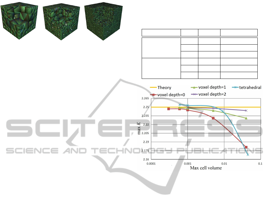
(a) 0.1 (b) 0.01 (c) 0.0005
Figure 9: Cross sections of tetrahedral meshes of the unit
cube. The maximal cell volume is indicated below each
figure.
minumum of kd f
v
· h
j
k sampled at random directions
h
1
,...,h
m
.
3.5 Results and Validation
We present results of numerical computations of qc-
dilatation for various domains and maps. We employ
the following default methods of computations, un-
less stated otherwise. Singular values are computed
from the estimation of Jacobian matrices, described in
subsection 3.4, while Jacobians are approximated by
a volume ratio (22). Solid angle weights were used for
tetrahedral meshes, and arithmetic average for voxel
meshes.
Figure 7 summarizes results for the Zorich map-
ping with a = 1 of the unit sphere, represented by
both voxel and tetrahedral meshes. One can notice
the correlation between areas on the surface of higher
values of qc-dilations and areas of higher values of
mean curvature and dihedral angles. From compari-
son of figures 7(e),7(f) with the figures 7(i),7(j), it is
obvious that gradient methods for singular values are
preferable over the methods of length ratios.
Figure 8 depicts no visible correlation between qc-
dilatations and Jacobian values, shown for parameter-
ization of the tetrahedral model.
To validate our approach we selected qc-mappings
with known dilatations and compared our numerical
results with the theoretical values. The simplest qc-
mappings were examined first. Estimations for a lin-
ear map showed the exact theoretical value for maxK
of the domain with the precision of 10
−5
. The same
accuracy was achieved for Jacobian and singular val-
ues at the chosen point. Folding map, which is a linear
map in cylindrical coordinates, also gave close results
to the theory, according to the table 2.
Figure 10 shows the relations that exist between
numerical estimation of maximal qc-dilatation K and
maximal cell size of a mesh. These computations
were performed for the same radial map on 2 domains
represented by different volumetric meshes. As ex-
pected, numerical estimations of max K converges to
the exact theoretical value as the maximal cell size
Table 2: Folding maps for different values of β/α were ap-
plied on tetrahedral and voxel meshes of the torus parallel to
xz plane, placed at (0,2,0). Voxel mesh is denoted according
to (10).
Mesh type β/α maxK Exact maxK
cubic(10;2;2)
0.5 3.996 4
1.5 2.249 2.25
2 3.997 4
Tetrahedral
0.5 4.01 4
1.5 2.264 2.25
2 4.063 4
Figure 10: Relation between max cell volume of volumet-
ric meshes, shown on a logarithmic scale, and accuracy of
the maxK computation. Voxel meshes were generated from
the torus surface with different depth values and a raising
number of divisions (see Fig. 4). Tetrahedral meshes were
generated from the surface of the unit cube with different
restrictions on the quality and on the maximal cell volume
(see Fig. 9). All the volumes were transformed by the ra-
dial map for a = 1.5, for which max K = 2.25 , as given by
equation (15).
approaches zero. This is basically due to the fact that
our estimates are based on piecewise linear approxi-
mations of f , which converge to f when the maximal
cell size goes to zero.
3.6 Quasi-conformal Coefficients
While there is an abundance of conformal mappings
in 2D, general volumetric domains can be mapped
only quasi-conformally. Therefore one of the chal-
lenges in 3D is to measure the minimal conformal dis-
tortion required to map one domain into another. The
corresponding quantity is called a quasi-conformal
coefficient of domains D and D
0
, and it is defined as
K(D,D
0
) = infK( f ) , (35)
where the infimum is taken over all qc-mappings
f : D → D
0
. The problem to compute K(D,D
0
) for
arbitrary domains, is generally unsolvable. There-
fore we should focus on lower bounds and specific
VolumetricQuasi-conformalMappings-Quasi-conformalMappingsforVolumeDeformationwithApplicationsto
GeometricModeling
55

3D domains. Our main interest will be qc-coefficient
K(D,B
3
), which corresponds to parameterizations of
volumes into the unit ball.
Volumes are generated from polygonal models
which, in fact, are surfaces of 3D polyhedrons. In-
tersections of adjacent faces of polyhedron forms 3D
wedges, which can be mapped by a similarity trans-
formation to
D
α
=

(r, ϕ, z) ∈ R
3


0 < ϕ < α, r > 0

, (36)
defined in cylindrical coordinates for some angle α.
Let’s define the following related notations.
Definition 3. A domain W is called a wedge of angle
α, If there exists a similarity transformation
S : W → D
α
.
Definition 4. A point b of a domain D is called a
wedge point of angle α, if b ∈ ∂D and there exists
neighbourhood U of b such that U ∩ W = U ∩ D,
where W is a wedge of angle α .
Suppose that qc-transformation f maps some
wedge point of angle α to a wedge point of angle β,
for 0 < α ≤ β ≤ π . V
¨
ais
¨
al
¨
a (V
¨
ais
¨
al
¨
a, 1971, pp. 132–
135) had concluded that in a small neighbourhood of
the wedge points, f behaves like a folding map de-
fined in (11). This fact implies the following inequal-
ity
K
I
( f ) ≥ β/α . (37)
Inequality (37) shows that in contrast to the 2D case,
there is no general conformal map between 3D wedge
points.
Consider the half-space D
π
. It can be mapped
into a ball by inversion in the unit sphere placed at
(0,0,−1). Since the composition with a conformal
map preserves qc-dilatations (V
¨
ais
¨
al
¨
a, 1971, p. 43),
we have
K(D,B
3
) = K(D,D
π
) (38)
and, if D has a wedge point of angle α, by (37)
K
I
(D,B
3
) ≥ π/α. (39)
According to (Caraman, 1974, p. 434), the maxi-
mal dihedral angle of a convex polyhedron P with m
faces is
(m − 3)π
m − 1
. (40)
This, along with (39), yields the simple estimation
K
I
(P,B
3
) ≥
m − 1
m − 3
. (41)
Moreover, (37) implies that the minimal possi-
ble qc-dilatation of the mapping between tetrahedral
meshes f : M → M
0
is the maximal ratio of dihedral
angles
max
] (( f (σ
i
), f (σ
j
))
] (σ
i
,σ
j
)
, (42)
taken over adjacent faces σ
i
,σ
j
of the surface of M.
In particular, for a parameterization onto a cube
K( f ) ≥ max
π/2
] (σ
i
,σ
j
)
, (43)
and for a parameterization onto a ball, we have
K( f ) ≥ max
π
] (σ
i
,σ
j
)
, (44)
since the half-plane and a ball are conformally equiv-
alent.
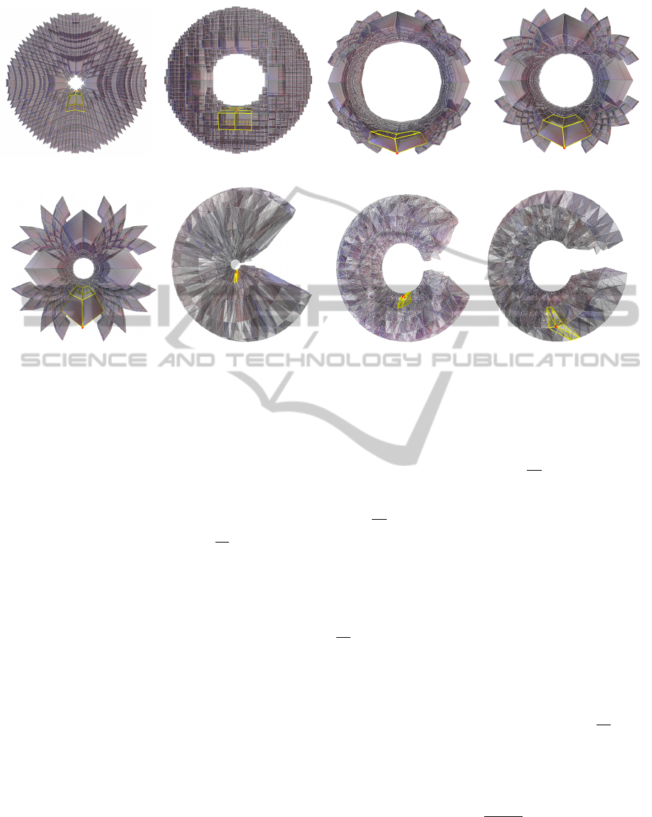
Figure 11 shows a series of convex polyhedrons
with raising number of faces. Each polyhedron was
mapped to B
3
by a radial stretching described in (20).
The resulting values of maximal dilatations K are con-
sistent with (41). As one can assert from the figure,
maximal values of K are obtained at boundary ver-
tices. These boundary vertices are the wedge points
that prescribe the lower bound for K
I
.
4 CONCLUSIONS
Deformations and parameterizations of discrete vol-
umes are employed in such areas of engineering and
science as Solid Modeling, MRI data processing etc.
Our quantitative method of computing qc-dilatations
provides a natural metric for estimation of the global
and local quality of volume deformation. This method
is readily available for comparison with other tech-
niques that are used in volumetric parameterizations,
e.g. discrete harmonic energy (Wang et al., 2003).
Among other applications, our approach can be
used to produce desirable deformations and param-
eterizations of 3D domains, by minimizing the maxi-
mal qc-dilatation under the given conditions.
The problem of parameterization of star-shaped
domains was studied by (Xia et al., 2010). We pre-
sented a simple technique for quasi-conformal param-
eterization of volumes into the unit ball. This tech-
nique is based on radial stretching of star-shaped do-
mains. It can be extended to more general domains,
such as a set of connected convex segments.
According to the obtained numerical results and
theoretical propositions, qc-dilatations are tightly re-
lated to distortion of such geometrical properties as
mean curvature and dihedral angles. Additional math-
ematical research is currently in progress with the
goal in mind of further theoretical interpretation of
this and related result.
GRAPP2015-InternationalConferenceonComputerGraphicsTheoryandApplications
56

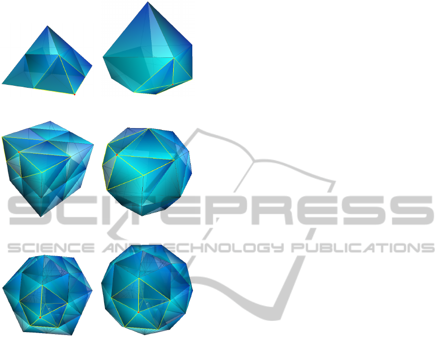
(a) 5 faces, max K = 12, average K = 4.7
(b) 6 faces, max K = 4.5, average K = 3.6
(c) 20 faces, max K = 1.8, average K = 1.5
Figure 11: Parameterization of convex polyhedrons, per-
formed by the radial stretching toward the unit ball, with
a = 1. Each figure shows, from left to right, tetrahedral
mesh of domain and image. Highlighted areas are the 1-
rings of the vertices that reached maximal dilatation. Keep
in mind, that parameterization is applied on vertices and it
does not refine meshes. Therefore the surface of the result-
ing image can deviate from being round.
ACKNOWLEDGEMENTS
Emil Saucan’s research was supported by Israel Sci-
ence Foundation Grants 221/07 and 93/11 and by Eu-
ropean Research Council under the European Com-
munity’s Seventh Framework Programme (FP7/2007-
2013) / ERC grant agreement n
o
[URI-306706].
The research of Y. Y. Zeevi is supported by the
Ollendorff Minerva Center for Vision and Image Sci-
ences.
REFERENCES
Ahlfors, L. V. (2006). Lectures on quasiconformal map-
pings. Providence, RI: American Mathematical Soci-
ety (AMS), 2nd enlarged and revised edition.
Almgren, F. J. and Rivin, I. (1999). The mean curvature
integral is invariant under bending. In The David Ep-
stein 60th birthday Festschrift. International Press.
Amanatides, J. and Woo, A. (1987). A fast voxel traver-
sal algorithm for ray tracing. In Eurographics ’87,
pages 3–10. Elsevier Science Publishers, Amsterdam,
North-Holland.
Caraman, P. (1974). n-dimensional quasiconformal (QCF)
mappings. Revised, enlarged and translated from the
Roumanian by the author.
Dukowicz, J. (1988). Efficient volume computation for
three-dimensional hexahedral cells. Journal of Com-
putational Physics.
Karabassi, E.-A., Papaioannou, G., and Theoharis, T.
(1999). A fast depth-buffer-based voxelization algo-
rithm. Journal of Graphics Tools: JGT, 4(4):5–10.
Lev, R., Saucan, E., and Elber, G. (2007). Curvature estima-
tion over smooth polygonal meshes using the half tube
formula. In Martin, R. R., Sabin, M. A., and Winkler,
J. R., editors, IMA Conference on the Mathematics of
Surfaces, volume 4647 of Lecture Notes in Computer
Science, pages 275–289. Springer.
Perreault, S. (2007). Octree C++ Class Template.
http://nomis80.org/code/octree.html.
Rickman, S. (1993). Quasiregular mappings, chapter 1,
page 15. Berlin: Springer-Verlag.
Si, H. (2009). A Quality Tetrahedral Mesh Generator and
Three-Dimensional Delaunay Triangulator. Tetgen,
http://tetgen.berlios.de.
V
¨
ais
¨
al
¨
a, J. (1971). Lectures on n-Dimensional Quasicon-
formal Mappings. Springer-Verlag Berlin Heidelberg
New York.
van Oosterom A, S. J. (1983). The solid angle of a plane
triangle. In IEEE Trans Biomed Eng.
Wang, Y., Gu, X., Yau, S.-T., et al. (2003). Volumetric har-
monic map. In Communications in Information & Sys-
tems, volume 3, pages 191–202. International Press of
Boston.
Willmore, T. (1993). Riemannian geometry. Oxford:
Clarendon Press.
Xia, J., He, Y., Han, S., Fu, C.-W., Luo, F., and Gu, X.
(2010). Parameterization of star-shaped volumes us-
ing green’s functions. In Mourrain, B., Schaefer, S.,
and Xu, G., editors, GMP, volume 6130 of Lecture
Notes in Computer Science, pages 219–235. Springer.
VolumetricQuasi-conformalMappings-Quasi-conformalMappingsforVolumeDeformationwithApplicationsto
GeometricModeling
57