
Unmixing of Hyperspectral Images with Pure Prior Spectral Pixels
Abir Zidi
1
, Julien Marot
2
, Klaus Spinnler
1
and Salah Bourennane
2
1
Fraunhofer IIS, Erlangen, Germany
2
Institut Fresnel, Marseille, France
Keywords:
Non-negative Matrix Factorization, PARAFAC, Linear Algebra, Hyperspectral Image, Remote Sensing,
Tensor.
Abstract:
In the literature, there are several methods for multilinear source separation. We find the most popular ones
such as nonnegative matrix factorization (NMF), canonical polyadic decomposition (PARAFAC). Inthis paper,
we solved the problem of the hyperspectral imaging with NMF algorithm. We based on the physical property
to improve and to relate the output endmembers spectra to the physical properties of the input data. To
achieve this,we added a regularization which enforces the closeness of the output endmembers to automatically
selected reference spectra. Afterwards we accounted for these reference spectra and their locations in the
initialization matrices. To illustrate our methods, we used self-acquired hyperspectral images (HSIs). The first
scene is compound of leaves at the macroscopic level. In a controlled environment, we extract the spectra of
three pigments. The second scene is acquired from an airplane: We distinguish between vegetation, water, and
soil.
1 INTRODUCTION
Unmixing is an important preprocessing step to fur-
ther analyze a hyperspectral image (HSI). Tensor de-
composition method has been adapted to unmix HSIs,
for instance PARAFAC model. However, this model
has problems: Firstly, PARAFAC algorithms are very
slow in certain circumstances. The alternating least
squares algorithm (ALS), used in the PARAFAC-
decomposition, may require a very large number of it-
erations before converging. This slowness of conver-
gence can result from large data, improper packaging,
or the presence of degeneration. Secondly PARAFAC
algorithms are very complicated to use. Indeed, there
are several parameters to find. In this paper, a new al-
gorithms developed with the purpose of circumvent-
ing these problems. It consists in decomposing a set
of spectra contained in a matrix Y as the following
product: Y = AX + N, where X is the endmember
matrix containing the ’source’ spectra, A is the mixing
matrix containing the mixing coefficients or contribu-
tion of each ’source’ or endmember, and N stands for
the modeling errors. Finding out an estimate
ˆ
A of the
mixing matrix, with the positivity and possibly sum-
to-one contraints, and an estimate
ˆ
X of the endmem-
ber matrix with the positivity constraint is a low-rank
approximation problem commonly called Nonnega-
tive Matrix Factorization (NMF) (H. Kim et al.,2008).
NMF has been applied to HSI data characteriza-
tion, and exhibited some advantages with respect to
existing endm ember extraction methods such as ver-
tex component analysis (VCA) (JMP. Nascimento et
al., April 2005). The interest of VCA was illustrated
in the frame of plant analysis in (J. Marot et al., June
2013). It turned out that, contrary to NMF, VCA does
not ensure the positivity of the mixing coefficients.
NMF has been extensively improved for the past few
years (A. Cichocki,et al.,2009). In (Ma et al., Jan-
uary 2004), spectral unmixing is related to optimiza-
tion and signal processing (in particular: convex ge-
ometry concepts). But despite its advantages, it still
exhibits some drawbacks: Firstly, it is sensitive to ini-
tialize (Q. Du, et al., July 2005). Secondly, there exist
an infinite number of solutions for A and X, and not
all of them bear a physical significance. Hence, our
problematic is two-fold: How to find an appropriate
initialization for the endmember matrix and for the
mixing matrix? How can we approach a solution with
a physical significance?
Firstly, we propose to use the purest spectra in
the scene, selected by a geometrical criterion (JMP.
Nascimento et al., April 2005), as a subset of ini-
tialization endmembers. As sources are often mostly
grouped in separate regions (H. Kim , et al.,2008),
we propose a sparse and positive initialization of the
mixing matrix, which accounts for the location of ini-
153
Zidi A., Marot J., Spinnler K. and Bourennane S..
Unmixing of Hyperspectral Images with Pure Prior Spectral Pixels.
DOI: 10.5220/0005311101530158
In Proceedings of the 10th International Conference on Computer Vision Theory and Applications (VISAPP-2015), pages 153-158
ISBN: 978-989-758-089-5
Copyright
c
2015 SCITEPRESS (Science and Technology Publications, Lda.)

tialization spectra.
Secondly, we propose to use the pure spectra
as references in the criterion which is minimized to
perform NMF. We expect that, as they are selected
among the spectral pixels of the HSI, aiming at the
closeness to these pure spectra will encourage the
physical significance of the endmembers provided by
NMF. That is why, for the first time to the best of our
knowledge, we introduce these spectra in the criterion
which is minimized for the purpose of factorization.
In Section 2, we present the notations which hold
throughout the paper, and we show how a HSI is han-
dled to get a set of one-dimensional spectra. The lin-
ear mixing model above is then detailed. In Section 3,
we propose an innovative initialization for the mixing
and endmember matrices, and a new criterion to per-
form NMF while ensuring the physical significance
of the estimated endmember spectra. In Section 4, we
detail our implementation of NMF. Section 5 presents
the results obtained: Firstly, we extract pigment spec-
tra from a leaf reflectance; secondly, we distinguish
between vegetated areas, soil and water in an aerial
HSI.
2 NOTATIONS AND DATA
MODEL
In the rest of the paper, x denotes a scalar, x denotes a
1-dimensional vector, X denotes a 2-dimensional ma-
trix, X denotes a multidimensional array, also called
”tensor” (D. Muti, et al., September 2008). For any
vector x, x
T
stands for transpose.
To set the link between algebraic methods and HSIs, a
HSI is considered from a mathematical point of view
as a tensor of order 3 T ∈ R
I
1
×I
2
×L
, where I
1
is the
number of rows, I
2
is the number of columns, and L
is the number of channels. In the following, we select
a subset of S ≤ I
1
I
2
spectral pixels of T and set them
row-wise in a matrix Y of size S × L.
Let’s consider one row of matrix Y, a spectral pixel
denoted by y
i
, which is a vector of size 1 × L. The
model that we adopt for y
i
is the linear combination
of J endmembers denoted by x
j
(j = 1,...,J). Vector
y
i
, i = 1, . . . ,S is expressed as:
y
i
=
J
∑
j=1
a
ij
x
j
+ n
i
(1)
where x
1
,x
2
,...,x
J
are the endmember spectra, and
a
i1
,a
i2
,...,a
iJ
stand for the abundances of each end-
member in the pixel vector y
i
.
The term n
i
stands for an additive residual term ac-
counting for the measurement noise and modeling er-
ror.
The endmember spectra are supposed to be positive-
valued. The abundances a
ij
, j = 1, . . . ,J are such that:
0 ≤ a
ij
≤ 1, ∀ i = 1,...,S (2)
J
∑
j=1
a
ij
= 1 ∀ i = 1, . . . , S (3)
Let a
i
= [a
i1
,a
i2
,...,a
ij
,...,a
iJ
] be the row vector
containing the abundance values associated with y
i
.
We define the abundance, or mixing matrix as A,
whose rows are the abundance vectors a
i
,i = 1, . . . , S
associated with the rows of matrix Y. We define the
endmember matrix as X, whose rows are the J end-
member spectra. With this formalism, and referring to
Eq. (1), we retrieve the linear mixing model presented
in the introduction. This data model is in agreement
with the one in (A. Cichocki, et al.,2009).
3 NEW CRITERION AND
INITIALIZATION MATRICES
FOR NMF
The basic NMF optimized function ensures that the
two matrix A and X are both nonnegatives. Since the
NMF solution is not unique, some prior knowledge
on HSIs can be introduced to solve this problem.
In this section, Accordance with valid knowledge
of the data, we add constraints (itemized in section 4)
to improve the result of deconvolution, using the pure
spectrum provided by an innovative initialization.
3.1 Minimized Criterion
To get an estimate of the endmember matrix and the
mixing matrix, we seek to minimize the criterion
D(Y||A,X):
ˆ
A,
ˆ
X = argmin
(A,X)
D(Y||A,X). In the sim-
plest versions of the NMF, assuming that the mod-
eling error N is independent identically distributed,
the problem of estimating A and X is formulated as
the maximization of a likelihood function (see (A. Ci-
chocki, et al.,2009), chapter 3), or equivalently, the
minimization of the criterion D
F
(Y||A,X) = ||Y −
AX||
2
F
, where ||· ||
F
denotes Frobenius norm. In real-
world data, the actual mixing matrix is rather sparse,
owing to the spatial repartition of the materials in the
scene: They are often grouped in regions. As advised
in (H. Kim et al.,2008), to induce sparsity in the mix-
ing matrix, we add an l
1
-norm regularization term. In
addition to this term which is related to the spatial
properties of the data, we also propose a regulariza-
tion term which is related to the shape of the spectra:
VISAPP2015-InternationalConferenceonComputerVisionTheoryandApplications
154

It enforces the endmembers to approach a set of so-
called ’pure’ spectra selected from the spectral pixels
of the HSI. This selection can be performed by vertex
component analysis, pixel purity index, or N-Finder
methods (JMP, et al.,April 2005). We choose ver-
tex component analysis because of its low complexity
(JMP, et al.,April 2005). Adding the spatial and the
spectral regularization terms yields:
D(Y||A,X) = ||Y−AX||
2
F
+α||A||
1
+β||X−X
pure
||
2
F
(4)
where matrix X
pure
’s rows are the J pure spectra, and
α and β are regularization coefficients.
3.2 Initialization Mmatrices
3.2.1 Endmember Matrix
Let J
′
≤ J be the number of spectra, among the rows
of matrix Y, which are assumed to result from a pure
material. Typically, one of these spectra can be issued
from the light reflected by a pure metal, or by a green
section of a leaf supposed to contain only chlorophyll.
We choose the first J
′
pure spectra provided by VCA
in subsection 3.1. Let X
1
Init
be the matrix whose rows
contain these spectra. The initialization endmember
matrix is defined as:
X
Init
=
X
1
Init
X
2
Init
(5)
where X
2
Init
is a random matrix compound of J − J
′
rows and L columns. Then, as explained in Sec-
tion 4, we scale each row of X
Init
to unit ℓ
2
norm
because we choose a hierarchical alternating least
squares (HALS) algorithm.
3.2.2 Abundance Matrix
Let k
1
,...,k
J
′
be the subset of row indices associated
with the initialization pure spectra
y
k
1
,...,y
k
J
′
in Y. The coefficients
a
ij
, for i = 1, ..., S, are
initialized as follows:
for j ≤ J
′
, a
ij
= 1 if i = k
j
; and a
ij
= 0 if i 6= k
j
for j > J
′
, a
ij
= 0 if i = k
j
; and a
ij
= λ if i 6= k
j
;
where, apart from λ < 1, we impose a sparsity
constraint: λ ≈ 1 for one value of i, and λ ≈ 0 for all
other values of i. Then, we scale each row of A to
unit sum. It is worth noticing that a factor 1 is set for
the location of each spectrum of X
1
Init
. For example,
with J = 5 and J
′
= 3:
A =
1 0 0 0 0
0.01 0.95 0.02 0.01 0.01
··· ··· ··· ··· ···
0.03 0.93 0.01 0.02 0.01
0 1 0 0 0
0 0 1 0 0
(6)
In Eq. (6), we choose solely coefficients which are
close to 0 or close to 1, to respect the sparsity con-
straint.
The criterion presented in this section is mini-
mized starting with the initialization matrices above,
with the algorithm whose implementation is detailed
in Section 4.
4 SPARSE HALS-NMF
IMPLEMENTATION
In this section, we present explanations of the criteria,
taking into account the physical realities, proposed in
the previous section and the implemented algorithm.
We propose a hierarchical implementation of the
combined generalized alternating least squares algo-
rithm proposed in (A. Cichocki, et al.,2009) (chapter
4). With a HALS scheme, we encourage the sparsity
of the mixing matrix and the smoothness of the end-
member spectra (A. Cichocki, et al.,2009).
Also, the HALS convergence speed outperforms the
one of projected gradient (W. Chen, et al., March
2012 ). However it is sensitive to the scaling of the
initial matrices (N. Gillis, et al., April 2010). For ex-
ample, as explained in (N. Gillis, et al., April 2010), if
the magnitude of the coefficients in the initial A and X
are not of the same order of magnitude as the values
in Y, this will lead to rank deficient approximations
and numerical problems.
The update rules derived from Eq. (4) are as follows:
X ⇐
A
T
Y+ βX
pure
||A||
2
F
+ β
(7)
A ⇐
YX
T
−
α
2
1
||X||
2
F
(8)
where 1 denotes a matrix with 1-valued coeffi-
cients.
Let ξ be a scalar whose magnitude is smaller than
any other value in the considered problem. We ensure
the non-negativity of any data ’d’ while performing
the following operation: d ← max[ξ,d]. In the fol-
lowing, we denote this operation as [d]
+
. The follow-
ing algorithm is a hierarchical implementation of the
update rules of Eqs. (7) and (8):
UnmixingofHyperspectralImageswithPurePriorSpectralPixels
155

Algorithm 1: HALS− NMF.
Set convergence parameter tol.
Initialize the criterion C to a large value.
Y is the observation matrix,
Add in Y a column of 1’s: Y = [1,Y].
Initialize X as in Eq. (5) and insert in X a column
of 1’s: X = [1,X].
Initialize A as in Eq. (6).
Set B = X
T
and B
pure
= X
T
pure
;
while C > tol do
update B:
W = Y
T
A;
V = A
T
A;
for j ∈ [1,J[ do
Update rule for b
j
(see Eq. (9))
end for
Update the columns of B as b
1
,b
2
,...,b
J
.
update A;
P = YB
Q = B
T
B
for j ∈ [1,J[ do
Update rule for a
j
(see Eqs. (10) and (11))
end for
Update the columns of A as a
1
,a
2
,...,a
J
.
Set X = B
T
;
Compute C = ||Y− AX||
2
F
.
end while
We use the term hierarchical because the columns
b
j
of matrix B and a
j
of matrix A are estimated suc-
cessively (see the two ’for’ loops in algorithm 1).
The update rule for b
j
is as follows:
b
j
⇐
b
j
+ w
j
− Bv
j
+ βb
pure
j
v
j j
+ β
+
(9)
where b
pure
j
refers to the columns of B
pure
.
The update rule for a
j
is as follows:
a
j
⇐
a
j
q
j j
+ p
j
− Aq
j
− α/2
q
j j
+
; (10)
a
j
⇐ a
j
/ka
j
k
2
(11)
The normalization in Eq. (11) helps mitigating the
effects of rotation indeterminacies on matrix A.
In the next section, we exemplify the proposed
method on hypespectral acquisitions of scenes con-
taining vegetation. We first consider artificial mix-
tures, and then spectra extracted from an aerial HSI.
5 RESULTS
This section presents some experiments performed on
data to illustrate the performance of the proposed non-
negative matrix factorization algorithm.
In the first place, we extract pigment spectra from
a leaf reflectance; afterwards, we distinguish between
vegetated areas, soil and water in an aerial HSI.
To achieve our acquisitions, we have based on
some facts: In (N. Dobigeon, et al., June 2013) , Do-
bigeon et. al. clearly emphasized the degradation of a
mixing model when the wavelengths of interest cover
both visible and infra-red (IR) domains:
Indeed, the pigment concentration rules the vege-
tation reflectance in the visible domain, whereas the
internal structure of the leaf does it in the IR domain.
We acquired HSIs with L=500 to 830 bands, between
400 and 700 to 900 nm: In the visible and the very
near IR domains. Some experiments permitted to rule
the regularization parameters to α = 0.2 and β = 0.6.
5.1 Artificial Spectral Mixtures
Figure 1a) presents three leaves with a homogeneous
color. We consider the content of these leaves as be-
ing as pure as possible, to get a first set of three refer-
ence spectra. These three spectra distinguish clearly
from each other: The green spectrum of Fig. 1b)
is the one of chlorophyll, also represented in (AK.
Mahlein et al., 2005), the yellow one is the spectrum
of carotenoid, which bears high values in the yellow
and orange wavelengths, the red spectrum is the one
of the anthocyanin. Indeed the red color of the leaf in
Fig. 1a) is characteristic of this phenolic compound,
that young leaves produce to protect themselves from
UV rays.
a)
50 100 150 200 250 300
20
40
60
80
100
120
140
160
180
200
400 500 600 700 800 900
0
0.1
0.2
0.3
0.4
0.5
0.6
0.7
0.8
0.9
1
Wavelength (nm)
Reflectance
b)
Figure 1: HSI data: a) three leaves with homogeneous color
containing pure pigments: chlorophyll, carotenoid, antho-
cyanin; b) spectra extracted from each leaf.
Starting from these three spectra, we create arti-
ficially mixed spectra. The mixing matrix is chosen
VISAPP2015-InternationalConferenceonComputerVisionTheoryandApplications
156
as:
A =
0 1.0000 0
0 0 1.0000
1.0000 0 0
0.7000 0.2000 0.1000
0.6000 0.2500 0.2500
0.2200 0.7000 0.0800
0.1000 0.6500 0.2500
0.1500 0.0100 0.8400
0.0300 0.0200 0.9500
0.9800 0.0100 0.0100
(12)
The estimated mixing matrix is:
ˆ
A =
0.0000 1.0000 0.0000
0.0252 0.0000 0.9748
0.8143 0.0594 0.1264
0.5688 0.2469 0.1843
0.4460 0.2633 0.2907
0.1755 0.7296 0.0949
0.0838 0.6680 0.2483
0.1427 0.0046 0.8527
0.0485 0.0059 0.9456
0.7979 0.0684 0.1336
(13)
One column corresponds to one endmember, and
one row to one location in the leaf. Figure 2 shows
the mixed and unmixed spectra. The unmixed spec-
tra are almost perfectly superimposed to the chosen
source spectra. The relative error between actual and
estimated spectra is 3.8%.
400 500 600 700 800 900
0
0.1
0.2
0.3
0.4
0.5
0.6
0.7
0.8
0.9
1
Wavelength (nm)
Reflectance
a)
400 500 600 700 800 900
0
0.1
0.2
0.3
0.4
0.5
0.6
0.7
0.8
0.9
1
Wavelength (nm)
Reflectance
b)
Figure 2: Mixed and unmixed spectra.
5.2 Vegetated Area Delimitation in
Aerial HSI
We now process an aerial HSI, that we acquired from
an airplane at the height of 500 meters. The spatial
resolution is as follows: 1 row accounts for 1 m., and
1 column accounts for 0.25 m. We choose S = I
1
I
2
:
we process all spectral pixels. The whole image is
provided at (Institut Fresnel). Fig. 3 shows the re-
sults obtained on a sub-image with 160 rows and 500
columns and L = 830 spectral bands. We fixed the
number of endmembers to four.
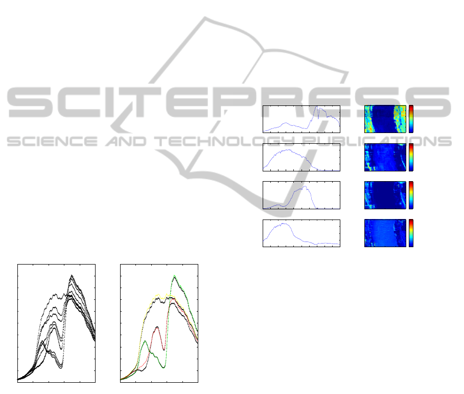
The left column in Fig. 3 presents the four es-
timated endmembers; the right column displays the
abundance maps from low contribution (blue) to high
contribution (red). The first endmember is similar in
shape to the spectrum of chlorophyll obtained in sub-
section 5.1. The gap around 760 nm is due to oxy-
gen absorbance. So we can assert that, in the re-
gions corresponding to abundance values above a cer-
tain threshold, such as 70%, the vegetation dominates.
The second endmember is associated with high abun-
dance values on the water of the river, and on the dirt
roads, from which we infer that it represents the spec-
trum of sunlight: It is most reflected in these regions
of the scene. The third endmember accounts for soil.
100 200 300 400
20
40
60
80
100
400 450 500 550 600 650 700 750 800 850 900
0
0.02
0.04
0.06
0.08
100 200 300 400
20
40
60
80
100
400 450 500 550 600 650 700 750 800 850 900
0
0.02
0.04
0.06
0.08
100 200 300 400
20
40
60
80
100
400 450 500 550 600 650 700 750 800 850 900
0
0.05
0.1
100 200 300 400
20
40
60
80
100
400 450 500 550 600 650 700 750 800 850 900
0
0.02
0.04
0.06
0.08
2
4
6
8
2
4
6
8
10
2
4
6
2
4
6
Figure 3: Estimated endmember spectra and abundance
map.
6 CONCLUSIONS
We consider unmixing of hyperspectral pixels by
NMF. We introduce spatial and spectral information
in the initialization mixing and endmember matri-
ces, and in the criterion which is minimized to per-
form NMF. For this, we select automatically with ver-
tex component analysis the purest spectra among the
spectral pixels. Firstly, these pure spectra are used as
a subset of initialization endmembers for NMF. The
mixing matrix is initialized as a sparse matrix, and
accounts for the location, in the HSI, of the initial-
ization endmembers. Secondly, we use the pure spec-
tra as references in a regularization term of the crite-
rion minimized for NMF. This term introduces some
spectral prior: It enforces the endmember spectra esti-
mated by NMF to exhibit some physical significance.
Apart from this term, which is the most novel as-
pect of this work, we use a second regularization term
UnmixingofHyperspectralImageswithPurePriorSpectralPixels
157

which accounts for a spatial prior knowledge on the
processed HSI: The materials in the scene are often
grouped in regions and consequently the mixing ma-
trix should be sparse, which is encouraged through its
l
1
-norm. We first imaged leaves, and then an aerial
partly vegetated scene. Considering their shape, the
proposed method permits to better interpret the end-
member spectra as a comparative implementation of
NMF. We could reliably delimitate the vegetated ar-
eas in remote sensing context.
ACKNOWLEDGEMENTS
The authors would like to thank the Bavarian Re-
search Foundation (BFS: Bayerische Forschungss-
tiftung) for supporting this researches done at the
Fraunhofer IIS in Frth.
We thank the firm ”Action Air Environnement”
for providing us with airplanes.
REFERENCES
H. Kim and K. Park, ”Non-negative Matrix Factoriza-
tion Based on Alternating Non-negativity Constrained
Least Squares and Active Set Method”, SIAM J.’l Ma-
trix Analysis and Applications, vol. 30(2), pp. 713-
730, 2008.
A. Cichocki, S. Amari, R. Zduneck, and A.H. Phan, ”Non-
negative Matrix and Tensor Factorizations: Appli-
cations to Exploratory Multi-way Data Analysis and
Blind Source Separation”, Wiley- Blackwell, 2009.
W. Chen and M. Guillaume, ”HALS-based NMF with
flexible constraints for hyperspectral unmixing”,
EURASIP Journal on Advances in Signal Processing,
vol. 2012(54), March 2012.
N. Dobigeon and C. Fevotte, ”Robust nonnegative matrix
factorization for nonlinear unmixing of hyperspec-
tral images,” IEEE WHISPERS, Gainesville, FL, June
2013.
Ma et al, ”A signal processing perspective on hyperspectral
unmixing”, IEEE Signal Processing Magazine, vol.
31(1), pp. 67-81, January 2014.
JMP. Nascimento and JMB. Dias, ”Vertex component anal-
ysis: a fast algorithm to unmix hyperspectral data”,
IEEE TGRS, vol. 43(4), pp. 898-910, April 2005.
J. Marot and S. Bourennane, ”Leaf marker spectra identifi-
cation by hyperspectral image acquisition and vertex
component analysis”, EUVIP’13, pp. 190-195, June
2013.
Q. Du, I. Kopriva, and H. Szu, ”Investigation on Con-
strained Matrix Factorization for Hyperspectral Im-
age Analysis”, In procs. of IEEE International Geo-
science and Remote Sensing Symposium, vol. 6, pp.
4304-4306, Seoul, July 2005.
N. Gillis and F. Glineur, ”Using underapproximations
for sparse nonnegative matrix factorization”, Pattern
Recognition, Vol. 43(4), April 2010, pp. 1676-1687.
P. O. Hoyer, ”Non-negative matrix factorization with
sparseness constraints”, Journal of Machine Learning
Research, vol. 5, pp. 1457-1469, 2004.
D. Muti, S. Bourennane, and J. Marot, ”Lower-Rank Tensor
Approximation and Multiway Filtering,” SIAM Jour-
nal on Matrix Analysis and Applications (SIMAX),
vol. 30(3), pp. 1172-1204, September 2008.
AK. Mahlein et. al, ”Recent advances in sensing plant
diseases for precision crop protection,” Eur J Plant
Pathol, vol. 133, pp. 197-209, May 2012.
John P. Kerekes et. al., ”SHARE 2012: subpixel detection
and unmixing experiments”, In Procs. SPIE 8743, Al-
gorithms and Technologies for Multispectral, Hyper-
spectral, and Ultraspectral Imagery, May 18, 2013.
http://www.fresnel.fr/perso/marot/Documents/
Aerial
HSI EUVIP.bmp
AK. Mahlein et. al., ”Hyperspectral Imaging for Small-
Scale Analysis of Symptoms Caused by Different
Sugar Beet Diseases”, Plant Methods, vol. 8, no 3,
pp. 1-13, 2012.
L. Chaerle et al., ”Multicolor fluorescence imaging for early
detection of the hypersensitive reaction to tobacco
mosaic virus,” Journal of Plant physiology, vol. 164,
pp. 253-262, March 2007.
VISAPP2015-InternationalConferenceonComputerVisionTheoryandApplications
158
