Convolutional Patch Networks with Spatial Prior for Road Detection and

Urban Scene Understanding

Clemens-Alexander Brust, Sven Sickert, Marcel Simon, Erik Rodner and Joachim Denzler

Computer Vision Group, Friedrich Schiller University of Jena, Jena, Germany

Keywords:

Convolutional Neural Networks, Patch Classiﬁcation, Road Detection, Semantic Segmentation, Scene

Understanding.

Abstract:

Classifying single image patches is important in many different applications, such as road detection or scene

understanding. In this paper, we present convolutional patch networks, which are convolutional networks

learned to distinguish different image patches and which can be used for pixel-wise labeling. We also show

how to incorporate spatial information of the patch as an input to the network, which allows for learning spatial

priors for certain categories jointly with an appearance model. In particular, we focus on road detection and

urban scene understanding, two application areas where we are able to achieve state-of-the-art results on the

KITTI as well as on the LabelMeFacade dataset.

Furthermore, our paper offers a guideline for people working in the area and desperately wandering through

all the painstaking details that render training CNs on image patches extremely difﬁcult.

1 INTRODUCTION

In the last two years, the revival of convolutional (neu-

ral) networks (CN) (LeCun et al., 1989) has led to a

breakthrough in computer vision and visual recogni-

tion. Especially the ﬁeld of object recognition and de-

tection made a huge step forward with respect to the

ﬁnal recognition performance as can be seen by the

success on the large-scale image classiﬁcation dataset

ImageNet (Krizhevsky et al., 2012). This break-

through was possible mainly due to two reasons: (1)

large-scale training data and (2) huge parallelization

to speed up the learning process. In general, an es-

sential advantage of CNs is the automatic learning of

task-speciﬁc representations of the input data, which

was previously often hand-designed.

While the majority of works focuses on applying

these techniques for object classiﬁcation tasks, there

is another ﬁeld where CNs can be really useful: se-

mantic segmentation. It is the task of assigning a class

label to each pixel in an image. This is why it is also

referred to as pixel-wise labeling. Previous works al-

ready showed how to use CNs in this area, e.g for road

detection (Alvarez et al., 2012; Masci et al., 2013).

However, the architectural choices and many critical

implementation details have not been discussed and

studied, although they are crucial for a high recogni-

tion performance. In our work, we therefore also give

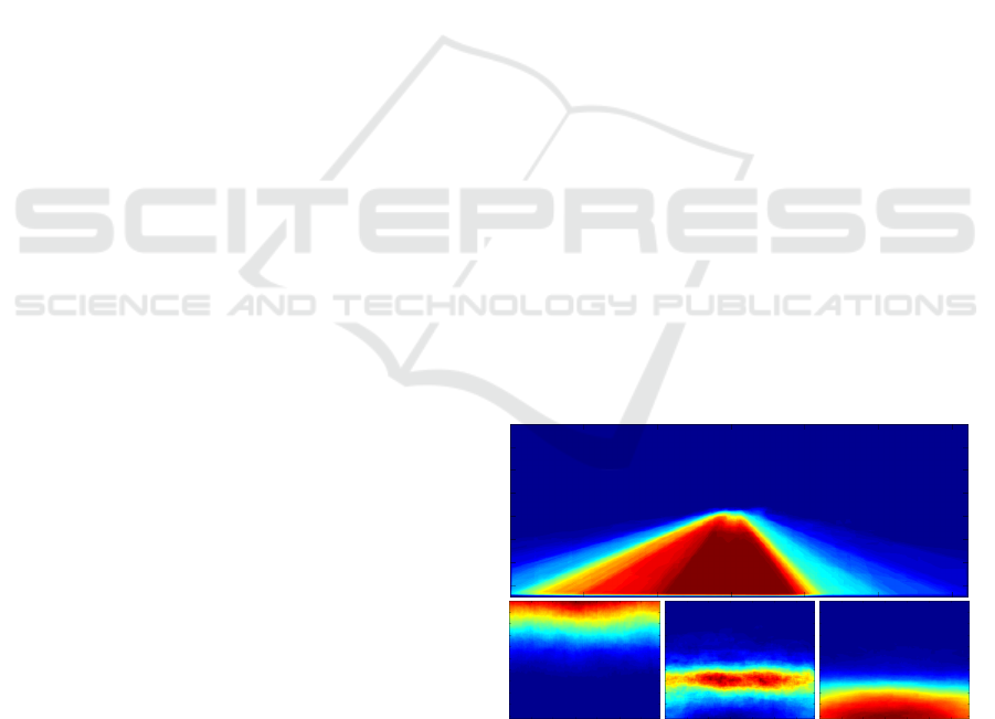
Figure 1: Illustration of spatial bias for categories in road

detection and urban scene understanding: (top) class road

of KITTI road challenge (Geiger et al., 2012), (bottom)

classes sky, car and road of LabelMeFacade (Fr

ohlich et al.,

2012). Warmer colors indicate higher probabilities (best

viewed in color).

a brief list of guidelines for CN training and discuss

several aspects important to get pixel-wise labeling

with CNs running.

Furthermore, we show how to learn spatial pri-

ors during CN training, because some classes appear

more frequently in some areas of an image (see Fig.

1). In general, predicting the label of a single pixel

requires a large receptive ﬁeld to incorporate as much

context information as possible. However, the high

510

Brust C., Sickert S., Simon M., Rodner E. and Denzler J..

Convolutional Patch Networks with Spatial Prior for Road Detection and Urban Scene Understanding.

DOI: 10.5220/0005355105100517

In Proceedings of the 10th International Conference on Computer Vision Theory and Applications (VISAPP-2015), pages 510-517

ISBN: 978-989-758-090-1

 2015 SCITEPRESS (Science and Technology Publications, Lda.)

input dimensionality would cause a huge CN model

with too many parameters for learning it robustly

while given only a small amount of training data. We

avoid this by incorporating absolute position informa-

tion in the fully connected layers of the CN.

In this paper, we use CN pixel-wise labeling for

the tasks of road detection and urban scene under-

standing. In road detection, the pixels of an image

are classiﬁed into road and non-road parts, which is

an essential task for autonomous driving. The chal-

lenge is the huge variability of road scenes, because

of changing light conditions, surface changes, and oc-

clusions. For a qualitative and quantitative evaluation,

we use the road estimation challenge of the popular

KITTI Vision Benchmark Suite (Geiger et al., 2012).

Urban scene understanding goes one step further by

increasing the number of categories that need to be

distinguished, such as buildings, cars, sidewalks, etc.

We obtain state-of-the-art performance in both do-

mains.

In the following, we ﬁrst give a brief overview of

the application of CNs for pixel-wise labeling. Sec-

tion 3 introduces our CN models and shows how to

learn spatial priors. Experiments are discussed and

evaluated in Section 4. A summary in Section 5 con-

cludes this paper.

2 RELATED WORK

Semantic segmentation was and is an active research

area with numerous publications. We will present

only those with relevant techniques (convolutional

neural networks or randomized decision trees) or a

similar scope of applications (road detection or urban

scene understanding).

Semantic Segmentation with CNs. The work of

(Couprie et al., 2014) presents an approach for seman-

tic segmentation with RGB-D images. The main idea

of their work is a multi-scale CN comprised of multi-

ple CNs for different scales of the images, which are

all linked to the fully connected layers at the end. In

contrast to their work, our approach incorporates the

spatial prior information as an important cue and a

possibility to learn a bias of the position of an object

in the image (Torralba, 2003).

Instead of performing semantic segmentation by

classifying image patches, (Gupta et al., 2014) builds

on algorithms for unsupervised region proposal gen-

eration. Each of the proposed regions is then classi-

ﬁed with an SVM that makes use of features learned

by CN using depth and geometric features as well as a

CN trained on RGB image patches. Similarly, (Hari-

haran et al., 2014) also classiﬁes object proposals and

combines a CN for detection and a CN for classify-

ing regions. In contrast to these works, we perform

pixel-wise labeling and are therefore not limited to a

few proposals generated by another algorithm.

Road Detection. Following up on their work with

slow feature analysis (K

uhnl et al., 2011), the au-

thors of (K

uhnl et al., 2012) propose spatial ray fea-

tures to ﬁnd boundaries of the road. The former work

serves as a source for base classiﬁers which model

road, boundary, and lanes. Especially the last one is

very important for the method, since ray features are

extracted from classiﬁer outputs. In contrast to our

work, this method strongly depends on the availabil-

ity of lane markings in the scene.

Another work in the ﬁeld aims at the problem of

changing light conditions in street scenes. In (Alvarez

and Lopez, 2011), the authors compute illumination

invariant images to segment the road even if the image

is highly cluttered due to shadows. Seeds are placed

in the bottom part of the illumination invariant image

where the road is supposed to be situated. All pixels

that have a similar appearance to the seeds will then

be classiﬁed as road. Since we learn local image ﬁl-

ters with the CNs, we do not have to explicitly model

illumination invariance in our approach but learn all

variations from the given dataset.

Similar to our approach, (Alvarez et al., 2012)

applied CNs for the task of road detection. How-

ever, their work focuses more on the transfer of la-

bels learned from a general image database which has

more images to learn from. Furthermore, they pro-

pose a texture descriptor which makes use of different

color representations of the image. Finally, general

information acquired from road scenes and informa-

tion extracted from a small area of the current image

are combined in a Naive Bayes framework to classify

the image.

Urban Scene Understanding. While road detec-

tion is a binary classiﬁcation scenario, the task of

urban scene understanding is to distinguish multiple

classes like car, building and sky.

In (Fr

ohlich et al., 2012) so-called iterative con-

text forests are used to classify images in a pixel-wise

or region-wise manner. The method is derived from

the well known random decision forests with the ad-

vantage that classiﬁcation results of one level of the

tree can be used in the next level as additional fea-

tures. The authors of (Scharwaechter et al., 2013)

also aim for the classiﬁcation of regions. They com-

bine appearance features of gray scale images and

ConvolutionalPatchNetworkswithSpatialPriorforRoadDetectionandUrbanSceneUnderstanding

511

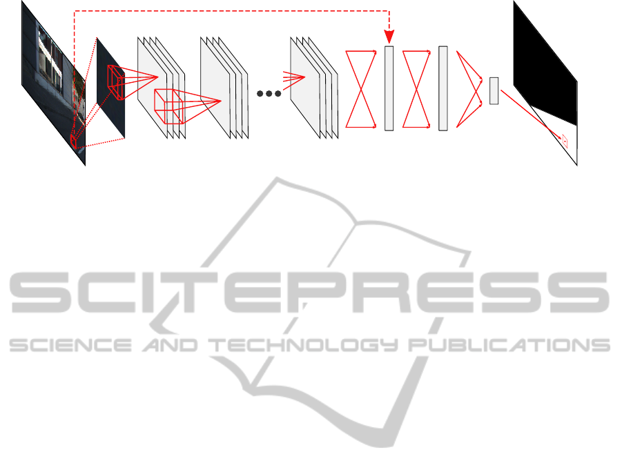
spatial information

input

image

convolutional, pooling

and non-linear activation layers

fully connected

layers

label estimation

for a single pixel

input

patch

Figure 2: Example of our convolutional patch network: in addition to the visual features we also incorporate the absolute

position information in the fully connected layers. The concrete architectures are given in the experimental section.

depth cues which are derived from dense disparity

maps. They incorporate a medium-level environment

model in order to obtain meaningful region hypothe-

ses. Then, a multi-cue bag-of-features pipeline is used

to classify these regions into object classes.

There are other works that incorporate additional

sources of information other than images from a sin-

gle camera. In (Zhang et al., 2010) dense depth maps

are used to compute view-independent 3D-features,

i.e. surface normal and height above ground. In con-

trast, the authors of (Kang et al., 2011) make use of

an additional near-infrared channel. They use hier-

archical bag-of-textons in order to learn spatial con-

text from the image. However, as these methods are

closely tied to a database that provides such informa-

tion, we propose a more generic approach.

3 CONVOLUTIONAL PATCH

NETWORKS

Convolutional (neural) networks (CNs) (LeCun et al.,

1989) belong to a family of methods, usually referred

to as “deep learning” approaches, especially in the

popular literature. The main idea is that the whole

classiﬁcation pipeline consists of one combined and

jointly trained model. Most recent deep learning ar-

chitectures for vision are based on a single CN. CNs

are feed forward neural networks, which concatenate

several layers of different types with convolutional

layers playing a key role.

3.1 Architecture and CN Training

The generic architecture of our CNs is visualized in a

simpliﬁed manner in Fig. 2. The input for our network

is always a single image patch extracted around a sin-

gle pixel we need to classify. Therefore, we use the

name Convolutional Patch Network for the method.

The network itself is structured in multiple layers.

Each convolutional layer convolves the output of the

previous layer with multiple learned ﬁlter masks. Af-

terwards, the outputs are optionally combined with a

maximum operation in a spatial window applied to the

result of each convolution, which is known as max-

pooling layer. This is followed by an element-wise

non-linear activation function, such as the hyperbolic

tangent or the rectiﬁed linear unit used in (Krizhevsky

et al., 2012).

The last layers are fully connected layers and mul-

tiply the input with a matrix of learned parameters

followed again by a non-linear activation function.

The output of the network are scores for each of the

learned categories or in the case of binary classiﬁca-

tion one score related to the likelihood of the positive

class. We do not provide a detailed explanation of the

layers, since this is described in many other papers

and tutorials (LeCun et al., 2001). In summary, we

can think about a CN as one huge model f (x;θ) that

tries to map an image through different layers to a use-

ful output. The model is parameterized by θ, which

includes the weights in the fully connected layers as

well as the weights of the convolution masks.

All parameters θ of the CN are learned by mini-

mizing the error of the network output for an example

compared the given ground-truth label y

θ = argmin

∑

i=1

·L ( f (x

;θ), y

) . (1)

In this setting L is a loss function and in our case we

use the quadratic loss.

Optimization is done with stochastic gradient de-

scent using momentum and mini-batches of 48 train-

ing examples (Krizhevsky et al., 2012). The learning

rate and all other hyperparameters are optimized on a

validation set.

VISAPP2015-InternationalConferenceonComputerVisionTheoryandApplications

512

optimization epochs

maxF performance (cross-validation) [%]

Tanh, heuristic initialization

Tanh, normalized initialization

ReLU, normalized initialization

ReLU, Dropout

Figure 3: Performance for road detection with respect to the

number of optimization epochs. The performance is mea-

sured by 10 times cross-validation on the KITTI training

set.

3.2 Incorporating Spatial Priors

As already motivated in the introduction and in Fig. 1,

predicting the category by using only the information

from a limited local receptive ﬁeld can be challenging

and in some cases impossible. Therefore, the work

of (Couprie et al., 2014) proposes a multi-scale CN

approach to incorporate information from receptive

ﬁelds with different sizes. In contrast, we exploit a

very common property in scene understanding. The

absolute position of certain categories in the image is

not uniformly distributed. Therefore, the position of

a patch in the image can be a powerful cue. This is

especially true for road detection as also validated by

(Fritsch et al., 2013).

Due to this reason, we provide the normalized po-

sition of a patch as an additional input to the CN. In

particular, the x ∈ [0, 1] and y ∈ [0, 1] coordinates are

added as inputs to one of the fully connected layers.

This can be viewed as having a smaller CN, which

provides a feature representation of the visual infor-

mation contained in the patch, and a standard multi-

ple layer neural network, which uses these features in

addition to the position information to perform clas-

siﬁcation. Whereas incorporating the position infor-

mation is a common trick in semantic segmentation,

with (Fr

ohlich et al., 2012) being only one example,

combining these priors with CN feature learning has

not been exploited before.

3.3 Software Framework

We implemented a new open source CN frame-

work speciﬁcally designed for semantic segmenta-

tion, which will be made publicly available.

The

source code was designed from scratch in C++11

aiming at multi-core architectures and not necessarily

strictly depending on GPU capabilities. An important

feature of the framework is the large ﬂexibility with

respect to possible CN architectures. For example, ev-

ery layer can be connected to an auxiliary input layer,

which is important in our case to allow for the incor-

poration of position information or to incorporate the

weight of a training example in the loss layer.

The framework does not depend on external li-

braries, which makes it practical, especially for fast

prototyping and heterogeneous environments. How-

ever, OpenCL or fast BLAS libraries such as ATLAS,

ACML, or Intel-MKL can be used to speed up con-

volutions and other algebraic operations. Convolu-

tions are in general realized by transforming them

into matrix-vector products, which requires some ad-

ditional memory overhead but leads to a signiﬁcant

speedup as also empirically validated by (Chellapilla

et al., 2006). For fast testing, the complete forward

propagation through the network can also be acceler-

ated by utilizing a device that computes OpenCL.

3.4 Important Details and

Implementation Hints

Implementing our own framework allowed us to have

inﬂuence on every aspect of the convolutional net-

work in order to apply it for the task of semantic seg-

mentation. Thereby, we made some important obser-

vations concerning parameter initialization and opti-

mization techniques.

Initialization of Network Parameters. The train-

ing of networks with many layers poses a particu-

lar challenge because of the vanishing gradient is-

sue (Glorot and Bengio, 2010). A repeated multipli-

cation of the derivatives produces smaller and smaller

values. This quickly leads to numerical problems

in deep networks, particularly when using single-

precision ﬂoating point calculations.

Usually, the weights in a layer with n inputs are

initialized randomly by sampling from a uniform dis-

tribution in [−

√

], which we refer to as heuristic

initialization. However, the authors of (Glorot and

This work was supported by Nvidia with a hardware

donation.

ConvolutionalPatchNetworkswithSpatialPriorforRoadDetectionandUrbanSceneUnderstanding

513

Bengio, 2010) analyze the effect of vanishing gra-

dients in detail and they derive an improved initial-

ization scheme, known as normalized initialization,

which has an important impact on the learning per-

formance. This can be seen in Figure 3, where we

plot the cross-validation accuracy of our road detec-

tion application after different numbers of optimiza-

tion epochs (an epoch are 10000 iterations with mini-

batches). As can be seen, the normalized initializa-

tion leads to a better performance of the network after

a few epochs.

Beneﬁt of Dropout and ReLU for Smaller Net-

works. Dropout as a regularizer is a means to pre-

vent a network from overﬁtting (Hinton et al., 2012),

which happens likely due to the large model complex-

ity of the networks. However, the small convolutional

net used in our approach for the task of road detection

does not beneﬁt from dropout as can be seen in Fig-

ure 3. Dropout has been shown to reduce error rates

signiﬁcantly in larger CN architectures (Krizhevsky

et al., 2012). Furthermore, Figure 3 also reveals that

using rectiﬁed linear units (Krizhevsky et al., 2012) as

nonlinear activations is beneﬁcial for the task of road

detection.

Task-speciﬁc Weighting of Training Examples. If

a recognition approach with a high performance with

respect to a task-speciﬁc performance measure is re-

quired, one should optimize with a learning objective

that comes as close as possible to the ﬁnal perfor-

mance measure. This hint might sound simple but we

give two examples in the following where this is ex-

tremely important to boost the performance.

For the KITTI Vision road detection benchmark,

performance is measured in the birds-eye view, while

data is presented in ego view. The authors of (Fritsch

et al., 2013) claim that the vehicle control usually hap-

pens in 2D space and therefore road detection should

also be done in this space. A wrong classiﬁed pixel

near the horizon in ego view represents a whole bunch

of pixels in the birds-eye view. To compensate for

this, we need to choose weights w

for the training

examples proportional to the size of the pixels after

transformation in the birds-eye view.

In urban scene understanding, we are faced with a

highly imbalanced multi-class problem, since pixels

labeled as building are more common than pixels la-

beled as door, for example. Therefore, performance is

usually measured in terms of accuracy (percentage of

correctly labeled pixels) and average recognition rate

(average of the class-wise accuracy) (Fr

ohlich et al.,

2012). To focus on the average recognition rate, we

weight examples according to their number of

examples in the training set, i.e. w

= n

−1

4 EXPERIMENTS

Our experiments in semantic segmentation are eval-

uated on two applications: road detection and urban

scene understanding, which are both challenging due

to the high variation of possible appearances within

the classes.

Figure 4: Convolution masks of the ﬁrst layer found during

learning on the KITTI road detection dataset.

4.1 Road Detection

For the task of road detection, we have to differenti-

ate between road and non-road patches and therefore

it is a typical binary classiﬁcation problem. In re-

cent years, the most commonly used road scene chal-

lenge is the KITTI Vision benchmark (Geiger et al.,

2012). This dataset features a multi-camera setup, op-

tical ﬂow vectors, odometry data, object annotations,

and GPS data.

There is a speciﬁc benchmark for road detection

with 600 annotated images where road and non-road

parts are labeled in the image. The dataset con-

sists of three different urban road settings: single-lane

roads with markings (UM), single-lane roads without

markings (UU) and multi-lane roads with markings

(UMM). There are challenges for road detection and

ego-lane detection. For this dataset, we follow the

evaluation protocol given in (Geiger et al., 2012) and

report the F1-measure as a binary classiﬁcation met-

ric which makes use of precision and recall such that

both have the same weight.

CN Architecture. We use the CN architecture

listed in Table 1 for road detection, where we classify

patches of size 28 ×28 extracted at each pixel loca-

tion. This architecture was optimized using ten-fold

cross validation. An important architectural choice

is the incorporation of the absolute position of the

patch as an input in layer 8. This allows for learn-

ing a spatial prior of the road category. Furthermore,

it is interesting to note that the ﬁrst layer applies con-

volution masks of a rather small size of 7 ×7. These

VISAPP2015-InternationalConferenceonComputerVisionTheoryandApplications

514

Figure 5: Qualitative results on the KITTI road detection dataset. Images show original input-data with labeled road pixels as

green overlay. Although a spatial prior is used in our approach we are able to segment road scenes with curves or occlusions

well. This ﬁgure is best viewed in color.

Table 1: CN architectures used for road detection (road det.)

and urban scene understanding (urban sun.) along with their

respective parameters. The number of outputs is denoted as

o. The parameters for a convolutional layer are given by

w ×h ×n, where n refers to the number of spatial ﬁlters

used, each of them with a size of w ×h. For pooling layers,

the parameters determine the spatial window for which the

maximum operation is performed.

# Type of layer Road det. Urban sun.

1 convolutional layer 7 ×7 ×12 7 ×7 ×16

2 maximum pooling 2 ×2 2 ×2

3 non-linear ReLU tanh

4 convolutional layer 5 ×5 ×6 5 ×5 ×12

5 non-linear ReLU tanh

6 fully connected layer o = 48 o = 64

7 non-linear ReLU tanh

8 fully connected layer o = 192 o = 192

+spatial prior

9 non-linear ReLU tanh

10 fully connected layer o = 1 o = 8

11 non-linear tanh sigmoid

Table 2: Results on the KITTI road detection dataset for

methods that only use the camera input image for predic-

tion.

Method MaxF

CN approach of (Alvarez et al., 2012) 73.97%

Spatial prior only (Fritsch et al., 2013) 82.53%

Spray features (K

uhnl et al., 2012) 88.22%

Our approach without spatial prior 76.34%

Our approach with spatial prior 86.50%

masks are visualized in Fig. 4 and depict certain tex-

tural and color elements that seem to be informative

when distinguishing between road and non-road im-

age patches.

Evaluation. The quantitative results of our road de-

tection approach are given in Table 2. We compare

with the method of (K

uhnl et al., 2012), which ob-

tains the current best result on the dataset, and the CN

method of (Alvarez et al., 2012). As can be seen, we

outperform the previous CN method by a large mar-

gin of over 10%. This can be mainly contributed to

the spatial prior we learn with the CN. How important

position information is for this dataset can be seen by

the performance of the baseline algorithm of (K

uhnl

et al., 2012) which uses only the pixel position during

testing without any appearance features.

As the qualitative results of our approach in Fig-

ure 5 show, we are able to segment curves although

a spatial prior is incorporated. This is due to the

weighting of these information which is automatically

learned in the training. When allowing a very high

weight for the spatial prior we would obtain similar

results to the baseline algorithm.

Note that we do not make use of any additional

information other than a single camera view. Some

competitors in the challenge incorporate data of the

second camera of the stereo setup or make use of the

3D point clouds from velodyne laser scanner. Their

results are not reported here but are given on the

KITTI website. At the time of submission we are on

place 4 of 22 in the ranking

4.2 Urban Scene Understanding

For urban scene understanding, each pixel is classi-

ﬁed into one of K classes. Our experiments are based

on the LabelMeFacade dataset (Fr

ohlich et al., 2012),

which consist of 945 images. The classes that need

to be differentiated are: building, window, sidewalk,

car, road, vegetation and sky. Furthermore, there is an

additional background class named unlabeled, which

we only use to exclude pixels from the training data.

Since this is a multi-class classiﬁcation problem, we

are following (Fr

ohlich et al., 2012) and use the over-

all recognition rate (ORR, plain accuracy) and the av-

erage recognition rate (ARR) which is the mean of

class-wise accuracies.

CN Architecture. For urban scene understanding,

we use the CN architecture reported in the right col-

umn of Table 1, which was also optimized with 50

training examples and 50 validation examples ran-

domly selected from the LabelMeFacade dataset. As

in the previous experiment, we extract patches of size

http://www.cvlibs.net/datasets/kitti/eval road.php, our

method is named CN24

ConvolutionalPatchNetworkswithSpatialPriorforRoadDetectionandUrbanSceneUnderstanding

515

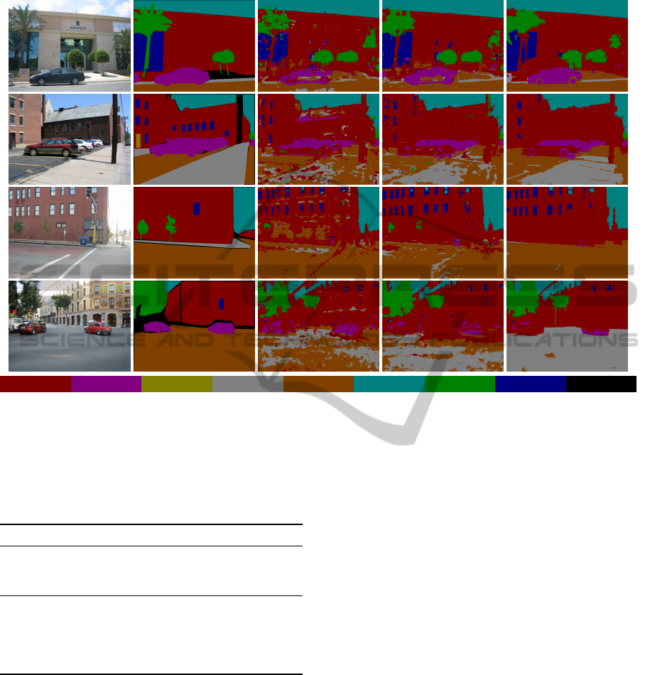
Original Ground-Truth pure CN outputs with spatial prior and post processing

building car door pavement road sky vegetation window unlabeled

Figure 6: Qualitative results for the LabelMeFacade dataset. We show results of our approach with and without adding

pixel positions as information for the learning procedure. As can be seen in the ﬁrst three rows, these additional information

improve the results (road vs. building). However, in some cases spatial priors do not help (pavement vs. road).

Table 3: Results on LabelMeFacade in comparison to pre-

vious work. We report overall and average recognition rates

for different networks. The weighted CN was optimized

with inverse class frequency weights.

Method ORR ARR

RDF+SIFT (Fr

ohlich et al., 2010) 49.06% 44.08%

ICF (Fr

ohlich et al., 2012) 67.33% 56.61%

RDF-MAP (Nowozin, 2014) 71.28% -

Our approach

pure CN outputs 67.87% 42.89%

+spatial prior 72.21% 47.74%

+post processing 74.33% 47.77%

+weighting 63.41% 58.98%

28 ×28 at each pixel location. In contrast to the CN

for road detection, we used the hyperbolic tangent

function as a non-linearity because it requires fewer

neurons to express anti-symmetric behavior.

Evaluation. As can be seen in Table 3, we are

able to achieve state-of-the-art performance on this

dataset. The spatial prior signiﬁcantly helps again to

boost the performance. Furthermore, we can directly

see that the weighting with respect to class frequen-

cies has a signiﬁcant impact on the ARR and the ORR

performance as already discussed in Sect. 3.4.

Four segmentation examples are shown in Fig-

ure 6 in comparison to the given ground-truth labels.

The authors of (Fr

ohlich et al., 2012) use a post-

processing step by fusing their results with an un-

supervised segmentation of the original images. The

probability outputs of the classiﬁer and the segments

are combined to ensure a consistent label within re-

gions. Since the output of our approach is scattered

due to the pixel-wise labeling (column 4 and 5), we

also added this post-processing step. We make use

of the graph-based segmentation approach of (Felzen-

szwalb and Huttenlocher, 2004) with parameters k =

550 and σ = 0.5. As can be seen in the last column

the results are improved with respect to object bound-

aries. However, this procedure can also lead to large

regions with a wrong labeling (row 4). Instead of road

the whole lower part of the image is classiﬁed as pave-

ment. Both classes have a very similar appearance in

most of the images.

5 CONCLUSIONS

In this paper, we showed how convolutional patch net-

VISAPP2015-InternationalConferenceonComputerVisionTheoryandApplications

516

works can be used for the task of semantic segmenta-

tion. Our approach performs classiﬁcation of image

patches at each pixel position. We analyzed differ-

ent popular network architectures along with differ-

ent techniques to improve the training. Furthermore,

we demonstrated how spatial prior information like

pixel positions can be incorporated into the learning

process leading to a signiﬁcant performance gain.

For evaluation, we used two different application

scenarios: road detection and urban scene understand-

ing. We were able to achieve very good results in the

road detection challenge of the popular KITTI Vision

Benchmark Suite. In this scenario we outperformed

several competitors, even those that use stereo images

or laser data.

For a second set of experiments, we used the

dataset LabelMeFacade of (Fr

ohlich et al., 2010)

which is a multi-class classiﬁcation task and shows

very diverse urban scenes. We were again able to

achieve state-of-the-art results. Future work will fo-

cus on speeding up the prediction phase, since we cur-

rently need around 30s for each image to infer the la-

bel at each position.

REFERENCES

Alvarez, J. M., Gevers, T., LeCun, Y., and Lopez, A. M.

(2012). Road scene segmentation from a single image.

In European Conference on Computer Vision (ECCV),

pages 376–389.

Alvarez, J. M. and Lopez, A. M. (2011). Road detection

based on illuminant invariance. IEEE Transactions on

Intelligent Transportation Systems, 12(1):184–193.

Chellapilla, K., Puri, S., Simard, P., et al. (2006). High

performance convolutional neural networks for docu-

ment processing. In Tenth International Workshop on

Frontiers in Handwriting Recognition.

Couprie, C., Farabet, C., Najman, L., and LeCun, Y. (2014).

Convolutional nets and watershed cuts for real-time

semantic labeling of rgbd videos. Journal of Machine

Learning Research (JMLR), 15:3489–3511.

Felzenszwalb, P. F. and Huttenlocher, D. P. (2004). Efﬁ-

cient graph-based image segmentation. International

Journal of Computer Vision, 59(2):1–26.

Fritsch, J., K

uhnl, T., and Geiger, A. (2013). A new per-

formance measure and evaluation benchmark for road

detection algorithms. In IEEE International Con-

ference on Intelligent Transportation Systems, pages

1693–1700.

ohlich, B., Rodner, E., and Denzler, J. (2010). A fast

approach for pixelwise labeling of facade images. In

Proceedings of the International Conference on Pat-

tern Recognition (ICPR), volume 7, pages 3029–3032.

ohlich, B., Rodner, E., and Denzler, J. (2012). Seman-

tic segmentation with millions of features: Integrat-

ing multiple cues in a combined random forest ap-

proach. In Asian Conference on Computer Vision

(ACCV), pages 218–231.

Geiger, A., Lenz, P., and Urtasun, R. (2012). Are we ready

for autonomous driving? the kitti vision benchmark

suite. In Computer Vision and Pattern Recognition

(CVPR), pages 3354–3361.

Glorot, X. and Bengio, Y. (2010). Understanding the dif-

ﬁculty of training deep feedforward neural networks.

In International Conference on Artiﬁcial Intelligence

and Statistics (AISTATS), pages 249–256.

Gupta, S., Girshick, R., Arbel

aez, P., and Malik, J. (2014).

Learning rich features from RGB-D images for object

detection and segmentation. In European Conference

on Computer Vision (ECCV).

Hariharan, B., Arbel

aez, P., Girshick, R., and Malik, J.

(2014). Simultaneous detection and segmentation. In

European Conference on Computer Vision (ECCV).

Hinton, G. E., Srivastava, N., Krizhevsky, A., Sutskever, I.,

and Salakhutdinov, R. R. (2012). Improving neural

networks by preventing co-adaptation of feature de-

tectors. arXiv preprint arXiv:1207.0580.

Kang, Y., Yamaguchi, K., Naito, T., and Ninomiya, Y.

(2011). Multiband image segmentation and object

recognition for understanding road scenes. IEEE

Transactions on Intelligent Transportation Systems,

12(4):1423–1433.

Krizhevsky, A., Sutskever, I., and Hinton, G. E. (2012). Im-

agenet classiﬁcation with deep convolutional neural

networks. In Advances in neural information process-

ing systems (NIPS), pages 1097–1105.

uhnl, T., Kummert, F., and Fritsch, J. (2011). Monocular

road segmentation using slow feature analysis. In Pro-

ceedings of the IEEE Intelligent Vehicles Symposium,

pages 800–806.

uhnl, T., Kummert, F., and Fritsch, J. (2012). Spa-

tial ray features for real-time ego-lane extraction. In

IEEE Conference on Intelligent Transportation Sys-

tems, pages 288–293.

LeCun, Y., Boser, B., Denker, J. S., Henderson, D., Howard,

R. E., Hubbard, W., and Jackel, L. D. (1989). Back-

propagation applied to handwritten zip code recogni-

tion. Neural computation, 1(4):541–551.

LeCun, Y., Bottou, L., Bengio, Y., and Haffner, P. (2001).

Gradient-based learning applied to document recogni-

tion. In Intelligent Signal Processing, pages 306–351.

IEEE Press.

Masci, J., Giusti, A., Ciresan, D. C., Fricout, G., and

Schmidhuber, J. (2013). A fast learning algorithm for

image segmentation with max-pooling convolutional

networks. arXiv preprint arXiv:1302.1690.

Nowozin, S. (2014). Optimal decisions from probabilis-

tic models: the intersection-over-union case. In Com-

puter Vision and Pattern Recognition (CVPR).

Scharwaechter, T., Enzweiler, M., Franke, U., and Roth, S.

(2013). Efﬁcient multi-cue scene segmentation. In

German Conference on Pattern Recognition (GCPR),

Lecture Notes in Computer Science, pages 435–445.

Torralba, A. (2003). Contextual priming for object de-

tection. International Journal of Computer Vision

(IJCV), 53(2):169–191.

Zhang, C., Wang, L., and Yang, R. (2010). Semantic seg-

mentation of urban scenes using dense depth maps. In

Daniilidis, K., Maragos, P., and Paragios, N., editors,

European Conference on Computer Vision (ECCV),

pages 708–721.

ConvolutionalPatchNetworkswithSpatialPriorforRoadDetectionandUrbanSceneUnderstanding

517