
A Comparison of Robust Model Predictive Control Techniques for a
Continuous Bioreactor
V. E. Ntampasi and O. I. Kosmidou
Department of Electrical and Computer Engineering, Democritus University of Thrace, 67100, Xanthi, Greece
Keywords:
Robust Model Predictive Control (RMPC), Uncertain Systems, Bioreactor, Bioprocess Control.
Abstract:
Biotechnology industry is expanded rapidly due to the progress in the understanding of bio-systems and the
increased demand for products. Since bioprocess dynamics are almost always affected by physical parameter
variations and external disturbances, the need for robust control techniques is of major importance in order
to ensure the desired behavior of the process. The overall process equilibrium is guaranteed if all quantities
in the bioreactor remain into prescribed ranges. In recent years, closed-loop control methods have been used
in order to cope with uncertainty and an important number of constraints imposed by the physical system.
For this purpose, predictive control is a quite promising technique. In the present paper three robust model
predictive control (RMPC) techniques are used in order to regulate the substrate concentration and the biomass
production in a bioreactor. These techniques are applied to a continuous bioreactor in which the pH changes
are considered as disturbances while the air pressure is ignored by the process model. For the simulation
purposes a linearized model of the system has been used in which the uncertainty is described in the form of
a disturbance term. The effectiveness of the methods is illustrated by means of simulation results.
1 INTRODUCTION
Since many physical systems can be modeled as un-
certain dynamic systems, methodologies and algo-
rithms related to the robust predictive control have
been developed during the last twenty years. Their
characteristics depend on marked differences in un-
certainty, performance criteria, the type of stability
constraints and calculation. In the sequel, some of
the basic principles that govern them are presented.
The RMPC was proposed in (Campo and Morari,
1987) based on min-max algorithms and since then
improved by several authors considering various sit-
uations (see e.g. (Allwright and Papavasiliou, 1992),
(Kothare et al., 1996a),(Scokaert and Mayne, 1998),
(Lee and Yu, 1997), (Kerrigan and Maciejowski,
2004) and related references). The min-max al-
gorithms generally do not promise robust stability;
to ensure the robust stability of the controlled sys-
tem, uncertainty should be variable with time (Zheng,
1995). The robust predictive control of stable linear
systems with constraints described by multiple mod-
els was solved in (Badgwell, 1997) by generalizing
the results in (Rawlings and Muske, 1993). In a differ-
ent context MOAS theory (Gilbert and Tan, 1991) was
developed for the reinforcement of strong restrictions
on predictive control situations, despite the presence
of input disturbances, by calculating the minimum re-
quired output horizon. Since then, the theory was fur-
ther developed (Mayne and Schroeder, 1997), (Bem-
porad, 1998), (Bemporad and Garulli, 1997), (A Cuz-
zola et al., 2002), (Mayne et al., 2006).
In recent years some new methods have been pro-
posed for robust predictive control: (i) In (Kothare
et al., 1996b), the so-called parametric approach was
proposed for the predictive control of linear uncertain
systems ensuring robust stability constraints. More-
over, it was noted that the cost function may be a
convex function of any type on the horizon forecast-
ing. The procedure guarantees closed loop stability
by using an LMI approach. Furthermore, the con-
struction of a standard computation algorithm in the
convex optimization framework has been proposed in
(Abate and El Ghaoui, 2004). (ii) Supervisory con-
trol was proposed in (Wang and Rawlings, 2004a),
(Wang and Rawlings, 2004b); this robust predictive
control methodology guarantees stability and offset-
free set point tracking in the presence of model un-
certainty. First, a min-max optimization is used to
determine the optimal control actions subject to the
input and the output constraints. A tree trajectory al-
lows forecasting time-varying model uncertainty. The
431
E. Ntampasi V. and I. Kosmidou O..
A Comparison of Robust Model Predictive Control Techniques for a Continuous Bioreactor.
DOI: 10.5220/0005480004310438
In Proceedings of the 12th International Conference on Informatics in Control, Automation and Robotics (ICINCO-2015), pages 431-438
ISBN: 978-989-758-122-9
Copyright
c
2015 SCITEPRESS (Science and Technology Publications, Lda.)

controller design procedure uses integrators to reject
disturbances and maintain the process at the opti-
mal operating conditions. (iii) A method based on
Quadratic Programming methods (QP) was presented
in (Schmid and Biegler, 1994); this method guaran-
tees stability and fast response to the set point in the
presence of model uncertainty.
In the present paper, these three above mentioned
approaches for robust predictive control are applied
to a bioprocess control system. They are chosen be-
tween different RMPC methods, since they are well
adapted to the precise problem formulation. Evalua-
tion and comparison of the three methods are based
on simulation results.
The paper is organized as follows: In Section II
the problem of RMPC for linear uncertain systems is
formulated. The effect of uncertainty is modeled as
a disturbance term. The parametric, supervisory and
QP approaches are presented in Sections III, IV and
V respectively. Then, they are applied to a bioreactor
process in Section VI. Finally, Section VII provides
concluding remarks.
2 ROBUST MODEL PREDICTIVE
CONTROL AND
DISTURBANCES
The robust model predictive control consists of ro-
bust analysis and robust synthesis. During the pro-
cess of analysis it is decided whether the system is
stable and meets the requirements of performance in
the presence of uncertainty of a given class. The syn-
thesis process leads to designing a controller such that
the controlled system remains robustly stable and sat-
isfies the requirements of robust performance. The
control algorithms differ in the type of uncertainty
characterizing the system and how one copes with it.
Hence, the resulting optimization procedures can in-
clude LMIs and dynamic programming.
In most cases, it is assumed that:
1. the nominal system belongs to S
0
, where S is a
given family of linear, time-invariant (LTI) sys-
tems and
2. a non-measured noise signal w(t) is introduced to
describe any type of uncertainty.
Consider a discrete-time linear system described by
the equations
∑
x
t+1|t
= Ax
t|t
+ Bu
t|t
+ Hw
t|t
y
t|t
= Cx
t|t
+ Kw
t|t
(1)
where w(t) ∈ W and is a given set. The uncertainty
may generally be either a parametric variation, or a
disturbance. The robust control scheme predicts the
systems behaviour in presence of uncertainty and ad-
justs the control signal with regard to the systems er-
rors.
3 THE PARAMETRIC
APPROACH FOR RMPC
In this section, the RMPC method proposed in
(Kothare et al., 1996b) is presented. The model of
a discrete-time LTI system is
x
t+k+1|t
= Ax
t+k|t
+ Bu
t+k|t
+ Hw
t+k|t
y
t+k|t
= Cx
t+k|t
h
x
t+k|t
,u
t+k|t
,w
t+k|t
≤ 0
x
t|t
= x
0
(2)
where t and k refer to time and future times, re-
spectively. The vectors: x
t
∈ X ⊂ R
n
, y
t
∈ R
r
and
u
t
∈ U ⊂ R
s
denote the state, measured outputs and
control inputs, respectively, while w
t
∈ W ⊂ R
q
is the
vector describing the disturbance inputs. A, B, C and
H are constant matrices of appropriate dimensions.
Since the system is subject to some physical limita-
tions, the sets X, U and W are determined to meet
inequality constraints of the form
x
L
≤ x
t+k|t
≤ x
U
u
L
≤ u
t+k|t
≤ u
U
w
L
≤ w
t+k|t
≤ w
U
,k = 0, 1,. ..,N
c
(3)
where N
c
is the control horizon and the superscripts
L and U refer to lower and upper bound, respec-
tively. Based on the following assumptions: (i) the
pair (A, B) is stabilizable (ii) the sets X, U and W
contain the equilibrium point and (iii) U and W are
compact sets, the RMPC is reformulated as an opti-
mization problem:
min
U=
{
u
t
,...,u
t+N
y
−1
}
J (U, x
t
)
x
t+k+1|t
= Ax
t+k|t
+ Bu
t+k|t
+ Hw
t+k|t
y
t+k|t
= Cx
t+k|t
h
x
t+k|t
,u
t+k|t
,w
t+k|t
≤ 0, k = 0,1, ...,N
c
x
t|t
= x
0
(4)
where J(U,x
t
) is the cost function and N
y
is the fore-
casting horizon of the output. The aim of control is
to ensure that the final state converges to the equilib-
rium point. More precisely, the method uses a Lya-
punov function to guarantee asymptotic stability of
the predictive control algorithm, based on the results
in (Keerthi and Gilbert, 1988). Therefore, the objec-
ICINCO2015-12thInternationalConferenceonInformaticsinControl,AutomationandRobotics
432

tive function is chosen to be of the quadratic form
J (U, x
t
) =
N
y
−1
∑
k=1
Qx
t+k|t
q
+
N
y
−1
∑
k=0
Ru
t+k|t
q
+
+
Px
t+N
y
|t
q
(5)
Then, the optimization problem is solved computa-
tionally by using a language for advanced modeling
and solution of convex and non-convex optimization
(Yalmip) (Lofberg, 2004),(L
¨
ofberg, 2008).
In the presence of a permanent disturbance, the
aim of control is modified and consists of ensuring
that the final state converges to an area as close to
the equilibrium point, as possible. For this purpose,
the above mentioned computation language has been
appropriately adapted, in the present paper.
4 THE SUPERVISORY
APPROACH FOR RMPC
In (Wang and Rawlings, 2004b) an RMPC method
is proposed to guarantee stability and offset-free set
point tracking in presence of model uncertainty. A
min-max optimization problem that explicitly ac-
counts for model uncertainty is used to determine the
optimal control actions subject to input and output
constraints. The robust regulator uses a tree trajec-
tory to forecast time-varying model uncertainty. The
controller design procedure uses integrators to reject
disturbances and maintain the process at the optimal
operating conditions or set points. Constraints may
cause offset, which occurs when the set points are un-
reachable. Finally, it should be noted that the method
considers polytopic system uncertainty, since this de-
scription can approximate many forms of uncertainty.
The method comprises a closed-loop stability con-
dition which requires the control to cope with un-
certainty. A novelty of the algorithm is to use a
tree diagram to predict the state of the system with
time-varying uncertainty. The control procedure is
achieved when all branches of the tree converge to
steady-state values of the state and control variables.
The uncertain dynamic system is described by the
following discrete state-space model:
∑
=
x
t+1
= A
t
x
t
+ B
t
u
t
y
t
= Cx
t
(6)
in which A
t
, B
t
are the time-varying state-space model
matrices of appropriate dimensions; C describes the
relationship between the output and the state in the
absence of uncertainty; as in the parametric method,
x
t
,y
t
and u
t
denote the state, measured outputs and
control inputs, respectively. When model uncertainty
is present, the exact plant model A
t
, B
t
is not known.
The model uncertainty region is described by the con-
vex hull Π =
{
(A
1
,B
1
),(A
2
,B
2
),..., (A
I
,B
I
)
}
. The
convex hull is defined as the linear convex combina-
tion of all models in Π . Let i, i = 1,2, ...,I be the
model index. (A
t
,B
t
) ∈ Π, if and only if there exist
µ
1
(t), µ
2
(t), ...,µ
I
(t) ∈ R, such that
A
t
=
I
∑
i=1
µ
i
(t)A
i
(7)
and
B
t
=
I
∑
i=1
µ
i
(t)B
i
(8)
for any [0 ≤ µ
i
(t) ≤ 1 and
I
∑
i=1
µ
i
(t) = 1. The system is
said to be at steady state at time T , if u
s
= u
s+1
= u(s),
x
s
= x
s+1
= x(s) and y
s
= y
s+1
= y(s), for all s ≥ T .
In the above relations,u
s
, x
s
and y
s
are the steady-state
control, state, and controlled output vectors, respec-
tively, that satisfy the constraints u
s
∈ U, x
s
∈ X and
y
s
∈ Y . Since there is no uncertainty in the output ma-
trix, y
s
= Cx is at steady state.
5 THE QP METHOD
The MPC technique used in the sequel consists of
minimizing
J (z, ε) = G
T
W
2
u
G + F
T
W
2
∆u
F + K
T
W
2
y
K + ρ
ε
ε
2
(9)
where z =
G F K
T
is the vector of optimiza-
tion variables with
G =
u(0)
·· ·
u(p − 1)
−
u
t arget
(0)
·· ·
u
t arget
(p − 1)
(10)
F =
∆u(0)
·· ·
∆u(p − 1)
(11)
K =
y(0)
·· ·
y(p − 1)
−
r (1)
·· ·
r (p)
(12)
Besides, the weight matrices W
u
, W
∆u
and W
y
are de-
fined as
W
u
= diag
w
u
0,1
,w
u
0,2
,. ..,w
u
0,n
u
,w
u
p−1,1
,
w
u
p−1,2
,. ..,w
u
p−1,n
u
(13)
W
∆u
= diag
w
∆u
0,1
,w
∆u
0,2
,. ..,w
∆u
0,n
u
,w
∆u
p−1,1
,
w
∆u
p−1,2
,. ..,w
∆u
p−1,n
u
(14)
AComparisonofRobustModelPredictiveControlTechniquesforaContinuousBioreactor
433

W
y
= diag
w
y
0,1
,w
y
0,2
,. ..,w
y
0,n
y
,w
y
p−1,1
,
w
y
p−1,2
,. ..,w
y
p−1,n
y
!
(15)
The parameters ε and ρ
ε
are a slack variable and its
weight, respectively; ρ
ε
penalizes the violation of the
constraints. As ρ
ε
increases with respect to the in-
put and output weights, the controller gives a higher
priority to minimization of constraint violations. The
u
target
is the set point for the input vector, p is the pre-
diction horizon, w
∗
i, j
are non negative weights for the
corresponding variables, r(k) is the current sample of
the output reference and are input increments (Rawl-
ings and Mayne, 2009), (Seborg et al., 2006). Finally,
after substituting u(k) , ∆u and y(k) in (9), it obtains
the form
J (z, ε) = ρ
ε
ε
2
+ z
T
K
∆u
z + 2z
T
r(1)
·· ·
r(p)
T
K
r
+
υ(0)
·· ·
υ(p − 1)
K
υ
+ u(−1)
T
+ K
u
+
u
t arget
(0)
·· ·
u
t arget
(p − 1)
K
ut
+ x(0)
T
K
x
z + c
(16)
where c is constrant. The last term is (16) introduces
the initial conditions into the minimization procedure.
The problem constraints are expressed in the terms of
(17) in which M
z
,M
ε
,M
lim
,M
u
,M
x
are constant ma-
trices of appropriate dimensions that depend on the
constraint bounds.
M
z
z + M
ε
ε ≤ M
lim
+ M
υ
υ(0)
·· ·
υ(p − 1)
+ M
u
u(−1)
+M
x
x(0)
(17)
Initially, the controller computes the optimal solution
z
∗
and ε
∗
by solving the quadratic program (QP) de-
scribed in (16)−(17).The model predictive controller
QP solver converts an MPC optimization problem to
the general QP form
min
x
f
T
x +
1
2
x
T
Hz
(18)
under constraints
ˆ
Ax ≤ b (19)
where x
T
=
z
T
ε
are the decisions, H is the Hes-
sian matrix,
ˆ
A is a matrix of linear constraint coeffi-
cients, b and f are vectors. The elements of H and
ˆ
A
are constant. The controller computes them during
initialization and retrieves them from the computer
memory when needed. It computes the time-varying
and vectors at the beginning of each control instant
(Rawlings and Mayne, 2009), (Seborg et al., 2006).
The MPC controller is implemented by using the
MPC control toolbox of Matlab. The toolbox uses the
KWIK algorithm to solve the QP problem (Schmid
and Biegler, 1994).
6 APPLICATION TO
BIOPROCESS CONTROL
Biotechnology industry is expanded rapidly due to
the progress in the understanding of bio-systems and
the increased demand for products (e.g. those widely
used in pharmaceutical and food industry, in various
chemical compounds etc). Their production is made
in special reactors called bioreactors. The main fea-
ture of a bioprocess consists of the material transfor-
mation procedure in presence of bacteria (or cells).
The incoming material concentration should be con-
trolled, such that it ensures the bacteria growth and
provide the desirable quantity of outgoing products.
The overall process equilibrium is guaranteed if all
quantities in the bioreactor remain into prescribed
ranges. Three types of bioreactors, namely batch,
fed batch and continuous, are mainly used. In this
paper the abovementioned robust model predictive
control techniques are applied to a continuous biore-
actor. In this process material quantities are con-
stantly added and removed to the reactor throughout
the fermentation. In most cases, bioreactor opera-
tion is based on empirical knowledge; however, in
recent years, closed-loop control methods have been
used (see e.g. (Rubio et al., 2001), (Mailleret et al.,
2004), (Fukushima and Bitmead, 2005), (Ashoori
et al., 2009) and related references).
Bioreactor systems are of increasing industrial
importance given their current use in pharmaceuti-
cals, bioremediation and specialty chemical produc-
tion. Although the majority of industrial bioprocess
operate in fed batch mode, a higher throughput could
be achieved in continuous operation. Unfortunately,
the biological organisms utilized in these reactors are
generally not well understood, and the cellular-level
metabolic pathways are poorly characterized. This
partial understanding makes advanced controller de-
sign difficult, as most advanced control techniques
utilize process models (Parker and Doyle, 1998). In
what follows, the RMPC approaches presented in
Sections 3, 4 and 5 are applied to a continuous biore-
actor in order to cope with uncertainty and an impor-
tant number of constraints imposed by the physical
system.
ICINCO2015-12thInternationalConferenceonInformaticsinControl,AutomationandRobotics
434

6.1 Description of the Process
The physical process in the bioreactor is modelled in
terms of non linear state-space equations (Freitas and
Teixeira, 1998), (Grossmann et al., 1983).
dx
dt
= [µ(s) − D]x
ds
dt
= −
1
Y
µ(s)s + D(S
a
− s)
(20)
with state variables,
• x(g/l): Cells concentration in the bioreactor
• s(g/l): Substrate concentration in the bioreactor
and time-varying parameters
• µ(s): Function that describes the cell growth
• D(1/h): Rate of dissolution
• Y : Yield coefficient of biomass
• S
a
(g/l): Incoming substrate concentration
The expression for µ(s) differs with respect to each
cell type. A common expression that has been experi-
mentally validated and used almost exclusively in the
literature is:
µ(s) =
µ
max
k
s
s
+ 1 + (
s
k
1
) + (
s
k
2
)
2
+ ... + (
s
k
n
)
n
(21)
where
• µ
max
: Constant
• k
s
: Constant of substrate saturation
• k
i
, i = 1,..., n: Constant parameters
For n = 0 one obtains the well-known Monod kinetics
µ(s) = µ
max
×
s
k
s
+ s
(22)
In the case where s takes large values with respect to
k
s
in (20), µ(s) becomes equal to µ
max
. As a result, the
differential equation (20) obtains the form
dx
dt
= λx (23)
where λ = µ
max
− D. In order to ensure a quite fast
bacteria growth, a positive value of λ has to be se-
lected.
Moreover, it is assumed that:
1. the volume of the bioreactor is constant and the
quantity of the incoming materials is equal to the
one of the outgoing materials
2. losses in temperature and changes into kinetic en-
ergy are neglected
3. pressure conditions, air supply, and the appear-
ance of unwanted gases are neglected.
6.2 RMPC Application
In this subsection, the parametric approach, the su-
pervisory approach and the QP for robust predictive
control are applied to a continuous bioreactor. The
RMPC objective is to maintain the substrate concen-
tration in the bioreactor almost constant (set point),
in order to produce the desired amount of biomass,
despite sharp decrease of pH, considered as a distur-
bance. It should be noted that an acid environment
in the bioreactor may cause inhibition of the bacteria
growth.
For the application purposes, a linearized model
of the process (20) is used describing the type of the
bioreactor
˙x = Ax + Bu + Hw
y = Cx
(24)
In the above model it is (Parker and Doyle, 1998)
A =
−2.564 −0.6792
1 0
(25)
B =
1
0
(26)
H =
1
1
(27)
C =
−1.5302 0.459
(28)
x
0
=
−1.530163
0.0174593
(29)
The performance index weighting matrices are
Q =
1 0
0 1
(30)
R = 10 (31)
and the set point is 15g/l.
The system is implemented by using the Yalmip
wiki (L
¨
ofberg, 2008) and the Model Predictive Con-
trol Toolbox of Matlab. Yalmip is a modeling lan-
guage for advanced modeling and solution of convex
and non-convex optimization problems. The main
motivation for using Yalmip is the rapid algorithm
development. Moreover, it can implement a large
amount of modeling tricks, allowing the user to con-
centrate on the high-level model, while Yalmip takes
care of the low-level modeling, in order to obtain effi-
cient and numerically sound models. For the simula-
tion purposes, the Yalmip wiki has been appropriately
adapted to cope with uncertainties in the form of de-
scription (24). The simulation results are obtained for
all cases (i) for the system without uncertainty and (ii)
for the system in presence of uncertainty.
AComparisonofRobustModelPredictiveControlTechniquesforaContinuousBioreactor
435
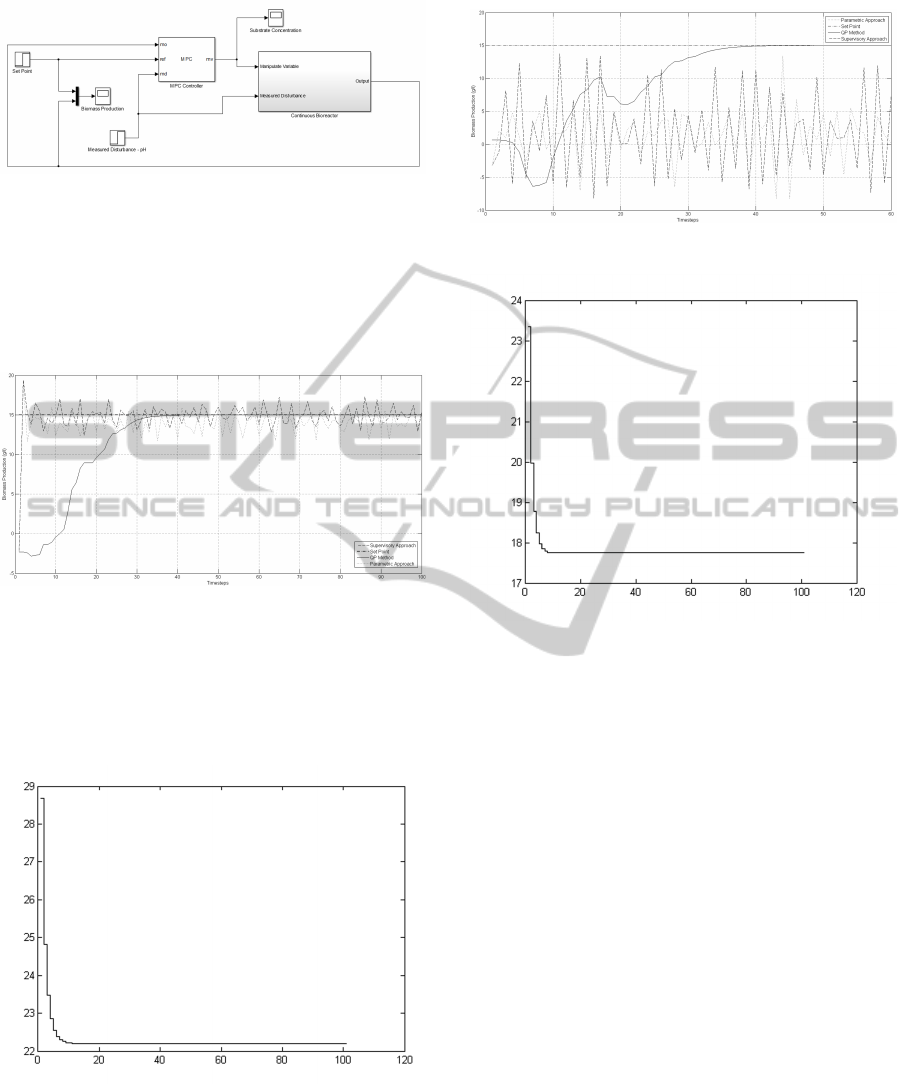
Figure 1: The simulation model in Simulink.
The simulation model in Matlab Simulink is given
in Fig. 1. We first consider the nominal system i.e.
without pH decrease. In this case the disturbance term
is neglected by the simulation algorithm. The systems
behavior is shown in Fig. 2 for the parametric, super-
visory and QP approaches.
Figure 2: RMPC of the nominal system in continuous biore-
actor.
Note that after 20 steps of the algorithm execution,
the QP method produces the desired biomass 15g/l
(set point), while the parametric and the supervisory
control do not. Fig. 3 shows that the substrate con-
centration with the QP method remains constant.
Figure 3: Substrate concentration for the QP method.
Consider now the case in which a sharp decrease
of pH occurs. The disturbance term is now taken into
account by the algorithm. The systems behaviour and
the substrate concentration obtained by the paramet-
ric, supervisory and QP approaches are shown in Fig.
4 and 5 respectively.
Figure 4: RMPC of the uncertain system in continuous
bioreactor.
Figure 5: Substrate concentration for the QP method.
Note the important overshoot due to the distur-
bance; it is also noted that, despite the pH decrease,
only the QP method ensures closed-loop systems sta-
bility. Furthermore, important fluctuations of the sub-
strate concentration are produced when the paramet-
ric and supervisory control methods are applied and
not in the QP one. However, it is considered that
the range of fluctuations is acceptable for the systems
equilibrium.
7 CONCLUSIONS
In this paper three robust predictive control ap-
proaches, namely parametric, supervisory and QP, are
used to the control of a bioreactor. The system is
generally nonlinear and uncertain due to pH changes.
Moreover, many physical constraints have to be met.
The control action has to ensure the overall process
stability and some desired level of performance, the
main design specification being a set-point of the sub-
strate concentration and biomass production. For the
simulation purposes a linearized model of the system
has been used in which the uncertainty is described in
the form of a disturbance term.
ICINCO2015-12thInternationalConferenceonInformaticsinControl,AutomationandRobotics
436

Comparison of the three methods based on sim-
ulation results has shown the following: 1) the QP
method allows to achieve the design objectives after a
small number of iterations, while both of the paramet-
ric and supervisory methods fail. 2) In the case when
a sharp decrease of pH occurs, the QP method is the
only one that ensures closed-loop systems stability. 3)
Application of the parametric and supervisory control
methods seem to produce important substrate concen-
tration fluctuations, in contrast to QP method. 4) Al-
though, due to the nature of the bioreactor, a certain
range of variations of the substrate concentration may
occur at the steady-state, the range of these variations
occurring by using the parametric and supervisory ap-
proaches is often not acceptable.
REFERENCES
A Cuzzola, F., C Geromel, J., and Morari, M. (2002). An
improved approach for constrained robust model pre-
dictive control. Automatica, 38(7):1183–1189.
Abate, A. and El Ghaoui, L. (2004). Robust model predic-
tive control through adjustable variables: an applica-
tion to path planning. In Decision and Control, 2004.
CDC. 43rd IEEE Conference on, volume 3, pages
2485–2490. IEEE.
Allwright, J. and Papavasiliou, G. (1992). On linear pro-
gramming and robust model-predictive control us-
ing impulse-responses. Systems & Control Letters,
18(2):159–164.
Ashoori, A., Moshiri, B., Khaki-Sedigh, A., and Bakhtiari,
M. R. (2009). Optimal control of a nonlinear fed-
batch fermentation process using model predictive ap-
proach. Journal of Process Control, 19(7):1162–1173.
Badgwell, T. A. (1997). A robust model predictive control
algorithm for stable linear plants. In American Control
Conference, 1997. Proceedings of the 1997, volume 3,
pages 1618–1622. IEEE.
Bemporad, A. (1998). A predictive controller with artificial
lyapunov function for linear systems with input/state
constraints. Automatica, 34(10):1255–1260.
Bemporad, A. and Garulli, A. (1997). Predictive control via
set-membership state estimation for constrained linear
systems with disturbances. In Proceedings of the 4th
European Control Conference.
Campo, P. J. and Morari, M. (1987). Robust model predic-
tive control. In American Control Conference, 1987,
pages 1021–1026. IEEE.
Freitas, C. and Teixeira, J. (1998). Hydrodynamic studies
in an airlift reactor with an enlarged degassing zone.
Bioprocess Engineering, 18(4):267–279.
Fukushima, H. and Bitmead, R. R. (2005). Robust con-
strained predictive control using comparison model.
Automatica, 41(1):97–106.
Gilbert, E. G. and Tan, K. T. (1991). Linear systems with
state and control constraints: The theory and appli-
cation of maximal output admissible sets. Automatic
Control, IEEE Transactions on, 36(9):1008–1020.
Grossmann, I. E., Halemane, K. P., and Swaney, R. E.
(1983). Optimization strategies for flexible chemi-
cal processes. Computers & Chemical Engineering,
7(4):439–462.
Keerthi, S. a. and Gilbert, E. G. (1988). Optimal infinite-
horizon feedback laws for a general class of con-
strained discrete-time systems: Stability and moving-
horizon approximations. Journal of optimization the-
ory and applications, 57(2):265–293.
Kerrigan, E. C. and Maciejowski, J. M. (2004). Feedback
min-max model predictive control using a single lin-
ear program: robust stability and the explicit solution.
International Journal of Robust and Nonlinear Con-
trol, 14(4):395–413.
Kothare, M. V., Balakrishnan, V., and Morari, M. (1996a).
Robust constrained model predictive control using lin-
ear matrix inequalities. Automatica, 32(10):1361–
1379.
Kothare, M. V., Balakrishnan, V., and Morari, M. (1996b).
Robust constrained model predictive control using lin-
ear matrix inequalities. Automatica, 32(10):1361–
1379.
Lee, J. a. and Yu, Z. (1997). Worst-case formulations of
model predictive control for systems with bounded pa-
rameters. Automatica, 33(5):763–781.
Lofberg, J. (2004). Yalmip: A toolbox for modeling and
optimization in matlab. In Computer Aided Control
Systems Design, 2004 IEEE International Symposium
on, pages 284–289. IEEE.
L
¨
ofberg, J. (2008). Modeling and solving uncertain opti-
mization problems in yalmip. In Proceedings of the
17th IFAC World Congress, pages 1337–1341.
Mailleret, L., Bernard, O., and Steyer, J.-P. (2004). Non-
linear adaptive control for bioreactors with unknown
kinetics. Automatica, 40(8):1379–1385.
Mayne, D. Q., Rakovi
´
c, S., Findeisen, R., and Allg
¨
ower,
F. (2006). Robust output feedback model predictive
control of constrained linear systems. Automatica,
42(7):1217–1222.
Mayne, D. Q. and Schroeder, W. (1997). Robust time-
optimal control of constrained linear systems. Auto-
matica, 33(12):2103–2118.
Parker, R. and Doyle, F. (1998). Nonlinear model predictive
control of a continuous bioreactor at near-optimum
conditions. In American Control Conference, 1998.
Proceedings of the 1998, volume 4, pages 2549–2553.
IEEE.
Rawlings, J. B. and Mayne, D. Q. (2009). Model predictive
control: Theory and design. Nob Hill Pub.
Rawlings, J. B. and Muske, K. R. (1993). The stability of
constrained receding horizon control. Automatic Con-
trol, IEEE Transactions on, 38(10):1512–1516.
Rubio, F. C., Garcia, J. L., Molina, E., and Chisti, Y. (2001).
Axial inhomogeneities in steady-state dissolved oxy-
gen in airlift bioreactors: predictive models. Chemical
Engineering Journal, 84(1):43–55.
AComparisonofRobustModelPredictiveControlTechniquesforaContinuousBioreactor
437

Schmid, C. and Biegler, L. T. (1994). Quadratic program-
ming methods for reduced hessian sqp. Computers &
chemical engineering, 18(9):817–832.
Scokaert, P. and Mayne, D. (1998). Min-max feedback
model predictive control for constrained linear sys-
tems. Automatic Control, IEEE Transactions on,
43(8):1136–1142.
Seborg, D., Edgar, T. F., and Mellichamp, D. (2006). Pro-
cess dynamics & control. John Wiley & Sons.
Wang, Y. J. and Rawlings, J. B. (2004a). A new robust
model predictive control method i: theory and com-
putation. Journal of Process Control, 14(3):231–247.
Wang, Y. J. and Rawlings, J. B. (2004b). A new robust
model predictive control method. ii: examples. Jour-
nal of Process control, 14(3):249–262.
Zheng, Z. Q. A. (1995). Robust control of systems subject
to contraints.
ICINCO2015-12thInternationalConferenceonInformaticsinControl,AutomationandRobotics
438
