A Unifying Polynomial Model for Efficient Discovery of Frequent
Itemsets
∗
Slimane Oulad-Naoui
1
, Hadda Cherroun
2
and Djelloul Ziadi
3
1
Département des Mathématiques et d’Informatique, Université de Ghardaia, Ghardaia, Algeria
2
Laboratoire d’Informatique et de Mathématiques, Université Amar Telidji, Laghouat, Algeria
3
Laboratoire LITIS - EA 4108, Normandie Université, Rouen, France
Keywords:
Data Mining, Frequent Itemsets, Formal Series, Weighted Automata, Algorithms, Unification.
Abstract:
It is well-known that developing a unifying theory is one of the most important issues in Data Mining research.
In the last two decades, a great deal has been devoted to the algorithmic aspects of the Frequent Itemset (FI)
Mining problem. We are motivated by the need of formal modeling in the field. Thus, we introduce and
analyze, in this theoretical study, a new model for the FI mining task. Indeed, we encode the itemsets as words
over an ordered alphabet, and state this problem by a formal series over the counting semiring (N, +,×,0,1),
whose the range constitutes the itemsets and the coefficients their supports. This formalism offers many advan-
tages in both fundamental and practical aspects: The introduction of a clear and unified theoretical framework
through which we can express the main FI-approaches, the possibility of their generalization to mine other
more complex objects, and their incrementalization and/or parallelization; in practice, we explain how this
problem can be seen as that of word recognition by an automaton, allowing an efficient implementation in
O(|Q|) space and O(|F
L
||Q|]) time, where Q is the set of states of the automaton used for representing the
data, and F
L
the set of prefixial maximal FI.
1 INTRODUCTION
Mining Frequent Itemsets (FI) is an important prob-
lem in Data Mining (DM). Although primitive,
it constitutes one of the most challenging and
over-two-decade-well-studied subject in the field.
Since the introduction of the Apriori algorithm by
Agrawal (Agrawal and Srikant, 1994), several algo-
rithms have been proposed to solve it. Without claim
of exhaustiveness, we can categorize these works
into three main classes, for more detail see (Hipp
et al., 2000; Goethals and Zaki, 2003; Han et al.,
2007): (i) Enumeration of all FI, (ii) Discovery of
closed/maximal FI, and (iii) Incremental algorithms.
The first class of algorithms aims to extract the
whole set of FI. The problem space exploration ap-
proaches used can be distinguished by the traver-
sal and the support calculation methods (Hipp et al.,
2000). In level-wise techniques, a breadth-first traver-
sal is adopted, where a k-itemset is derived by ex-
tending a frequent one of length k − 1 (Agrawal and
∗
This work is supported by the MESRS-Algeria under
the project number 8/U03/7015
Srikant, 1994). The calculation of the support of an
itemset is performed by database scans. In these tech-
niques, the most remarkable is, undeniably, the A-
priori heuristic used to prune the problem space, and
widely used in all algorithms later. Unfortunately,
these techniques suffer from two major drawbacks:
Generating a huge number of candidates, and an ex-
cessive I/O cost needed for support counting.
In (Zaki, 2000), the author considered the data
from a vertical angle of view, where he associated
with each itemset X its list of transactions (tidlist) and
uses set intersection for support calculation, which
has proven to be a more effective trick. However, and
despite the common-prefix equivalence relation pro-
posed to decompose the problem, this approach re-
quires, in dense datasets particularly, a large time and
intermediate memory to perform intersections.
In order to reduce the size of the dataset and
avoid multiple scans of it, Han et al. introduced the
FPGrowth algorithm (Han et al., 2004) that uses a
compact structure called Frequent-Pattern Tree (FP-
Tree) enhanced with the itemset supports. This al-
gorithm generates recursively a grown-pattern condi-
tional database projections for which a correspond-
49
Oulad-Naoui S., Cherroun H. and Ziadi D..
A Unifying Polynomial Model for Efficient Discovery of Frequent Itemsets.
DOI: 10.5220/0005516200490059
In Proceedings of 4th International Conference on Data Management Technologies and Applications (DATA-2015), pages 49-59
ISBN: 978-989-758-103-8
Copyright
c
 2015 SCITEPRESS (Science and Technology Publications, Lda.)

ing FPTrees are also constructed. Though, the perfor-
mance gain shown, the original version of FPGrowth
induces, sadly, an abundant memory and time over-
head due to repetitive sorting and reconstructions.
The algorithms of the second class focus on the
minimum set of FI, called the cover, which allows to
generate all the rest (Pasquier et al., 1999). Thereby,
the closed and maximal FI notions have been intro-
duced. These approaches use Formal Concept Analy-
sis (FCA) (Wille, 1982) to extract the set of frequent
concepts, that constitutes a condensed representation
of the entire set of FI.
The concern of the algorithms of the third class
was the incrementality. That is, how to generate
the set of FI, and to maintain it in the case of dy-
namic datasets (Valtchev et al., 2008). Here, the same
philosophies were adopted in either algorithmic fash-
ion or using FCA.
Summing up, after more than two decades of ac-
tive research on the subject, with countless techniques
including various efficient algorithms and judicious
data structures each with its benefits and drawbacks,
we believe that it will be convenient to go back and
ask a key question: Besides the existing ones (Godin
et al., 1995; Zaki and Ogihara, 1998), are there other
formalisms for this basic problem ? In other words,
we aim to develop a general unifying model able to
express the works done so far in the main state of the
art approaches. We wish, moreover, that the proposed
formalism should enjoy some capitals characteristics
such as : the completeness while remaining simple
and intuitive, extensibility, and efficiency. That is,
provide, why not, an implementation having a better
performances, if not stand at least comparable to those
of the existing techniques.
The elaboration of unifying models is a well-
established issue in DM (Yang and Wu, 2006). We
postulate that the unification can be facilitated if we
focus on a particular DM-task. In this paper, we ad-
dress this question for the FI-mining problem. In-
deed, we introduce a new model for enumerating all
FI based on formal series, which meets the above pro-
prieties. First, it defines a unified theoretical frame-
work, which leads to see the equivalence of the al-
gorithms as stipulated in (Goethals and Zaki, 2003)
and confirmed in one of the early comparative stud-
ies (Hipp et al., 2000). Second, it allows their gener-
alization for mining more complex objects. We prove
also a natural decomposition scheme, often required
in many aspects of the problem such that incremen-
tality or parallelization. Moreover, we explain how
this problem can be transposed to that of the realiza-
tion of a formal series by a weighted automaton (Sa-
lomaa et al., 1978), and consequently, to that of word
recognition, which is a largely invested topic with a
very mature algorithmic. Finally, we propose an ef-
ficient algorithm to enumerate all FI, which runs in
place without extra memory.
The remaining of this paper is organized as fol-
lows. We begin, in Section 2, by some preliminaries
on the basic concepts and notions to be used through-
out this article. In Section 3, we recall the FI mining
problem, and introduce our model. Section 4 is de-
voted to the definition, the proofs, the construction of
the proposed automaton, and the analysis of the min-
ing algorithm. In Section 5, we discuss our model
against the existing techniques and show how these
can be derived from it, and conclude in Section 6 with
some extensions.
2 PRELIMINARIES
A set M with an associative binary internal opera-
tion ∗ admitting a unique e ∈ M as an identity ele-
ment forms a structure of monoid, which we denote
(M,∗,e). When the operation ∗ is also commutative
then the monoid is commutative. The popular exam-
ple is the free monoid A
∗
of the set of words over an
alphabet A equipped with the concatenation of two
words, and having the empty word ε as an identity
element.
A word u is a prefix (respectively a suffix) of a
word w if there exists a word v such that w = uv
(respectively w = vu). The set of the prefixes of a
word u will be denoted Pref(u). This concept can
be extended to a set of words by performing the
union of the prefixes of its elements. A word u =
u
1
... u
k
is a subsequence of a word w = w
1
... w
l
(k ≤
l) if there exist words v
1
,.. .,v
k+1
, such that w =
v
1
u
1
v
2
u
2
... v
k
u
k
v
k+1
. We write then u 4 w.
A semiring is a tuple (K,+,×,0,1) such that:
(K,+,0) is a commutative monoid, (K,×, 1) is a
monoid, × distributes on both sides over +, and 0 is
an absorbing element with respect to ×. Examples
of semirings are (N,+,×,0,1) of positive integers,
(B,∨,∧, ⊥,>) of booleans, and the tropical semiring
(N ∪ {∞},min,+, ∞,0).
Over the monoid A
∗
, we define a formal series
S
with coefficients in a semiring K as a mapping
S
:
A
∗
→ K, which associates with each w its coefficient
h
S
,wi. The series
S
itself will be written as a sum:
S
=
∑
w∈A
∗
h
S
,wiw (2.1)
The set range(
S
) = {w ∈ A
∗
| h
S
,wi 6= 0} of words
with non-null coefficients is called the range of the
series
S
(also called its support, but we prefer range
DATA2015-4thInternationalConferenceonDataManagementTechnologiesandApplications
50

to avoid the confusion with the support of an itemset).
The set of formal series over A with coefficients on
K is denoted KhhAii. A structure of a semiring is
defined on KhhAii as follows,
S
and
T
are two formal
series on A with coefficients in K:
h
S
+
T
,wi = h
S
,wi + h
T
,wi (2.2)
h
S T
,wi =
∑
uv=w
h
S
,uih
T
,vi (2.3)
The subset of the series of KhhAii with finite range
are called polynomials and denoted by KhAi. There-
after, in the case of the monoid A
∗
, and for its identity
element ε, and for all k ∈ K we write kε (or simply k)
the term having k as coefficient of ε. In the same way,
for a word w on A
∗
, we denote kw (respectively w) the
term whose coefficient for w is k (respectively 1).
A weighted automaton A over an alphabet A
with coefficients in a semiring K is a tuple A =
(Q,A,µ, λ,γ), where Q is the finite set of states, µ the
function from Q to K of the initial (input) weights,
λ the function from Q × A × Q to K of the transition
weights, and γ the mapping from Q to K of the fi-
nal (output) weights. A path c in A is a succession
of transitions: (q
0
,a
1
,q
1
).. .(q
n−1
,a
n
,q
n
) labeled by
the word a
1
... a
n
obtained by the concatenation of the
symbols of its edges. Its weight is the product of the
weights of its transitions:
ω(c) = µ(q
0
)λ(q
0
,a
1
,q
1
).. .λ(q
n−1
,a
n
,q
n
)γ(q
n
)
(2.4)
If we denote by C (u) the set of all paths labeled u.
The weight of a word u in the automaton A, denoted
A(u), is the sum of the weights of the elements of
C (u):
A(u) =
∑
c∈C (u)
ω(c) (2.5)
The size of an automaton is the number of its transi-
tions.
3 PROBLEM STATEMENT AND
NOTATIONS
First, let us recall the basic concepts of the FI mining
problem, and introduce the definitions and notations
used throughout this paper.
Let A = {a
1
,a
2
,.. .,a
m
} be an alphabet of m sym-
bols called items. Those can designate, according to
the application domain, a products purchased from
a supermarket, a visited Web pages, a collection of
attributes.. .etc. An itemset is a subset of A, if k is its
cardinal it is called a k-itemset. A transaction t
i
is a
nonempty set of items identified by its unique identi-
fier i. A dataset D is a set of n transactions, which we
denote as a multi-set: D = {t
1
,t
2
,.. .,t
n
}. In a dataset
D, the support of an itemset x, denoted sprt(x,D), is
the number of transactions containing x, i.e :
sprt(x,D) = |{t
k
∈ D | x ⊆ t
k
}| (3.1)
An itemset x is frequent if its support exceeds a spec-
ified minimum support-threshold s. That is, x is fre-
quent in D if and only if sprt(x,D) ≥ s. A frequent
itemset is maximal if an only if there is no superset
of it which is frequent. The problem of mining FI
consists to discover the set F of all itemsets whose
support is greater than the given minimum support-
threshold s.
3.1 The Polynomial Model
Now, we show how to translate the FI mining problem
to the formal series model. Taking into account the
finiteness of the modeled data (itemsets and datasets),
we adopt thus a modeling based on polynomials.
The main idea in this modeling is to encode an
itemset by a word, and all its subsets by a polyno-
mial. After defining the polynomial of a dataset, the
question is then to extract from this polynomial all the
terms where the support-criterion holds.
First, let us assume, without loss of generality, that
the alphabet A is sorted according to an arbitrary total
order, where we can write:
A = {a
1
,a
2
... a
m
}, with: ε < a
1
< a
2
< ... < a
m
.
We represent a k-itemset x = {a
i
1
,a
i
2
,.. .,a
i
k
} by the
word w(x) of length k, built by the concatenation of
its items according to the predefined order. We will
write:
w(x) = a
i
1
a
i
2
... a
i
k
, such that a
i
1
< ... < a
i
k
(3.2)
In what follows, we confuse an itemset x and its word
representation w(x). That is, instead of x = {a, b,c},
we write simply x = abc. Note that the empty itemset
/
0 is represented by the empty word ε of length zero
(|ε| = 0).
Definition 3.1 (Itemset Subsequence Polynomial).
Let x = a
i
1
a
i
2
... a
i
k
be a k-itemset, The subsequence
polynomial S
x
associated with x is defined as follows:
S
x
= (a
i
1
+ 1)(a
i
2
+ 1) ...(a
i
k
+ 1), with: S
ε
= 1
(3.3)
Hereafter, we denote, for each a ∈ A, by
a the
polynomial (a + 1). So, the polynomial S
x
associated
with a k-itemset x will be denoted: S
x
= a
i
1
a
i
2
... a
i
k
.
So, S
x
is the polynomial that represents all the subsets
of x. For example, we associate with the itemset x =
AUnifyingPolynomialModelforEfficientDiscoveryofFrequentItemsets
51

abc the polynomial S
x
= abc = (a + 1)(b + 1)(c + 1),
that gives us the polynomial: 1 +a+b+c+ab+ac +
bc + abc.
From the itemset subsequence polynomial, we can
derive the subsequence polynomial associated with a
dataset D.
Definition 3.2 (Dataset Subsequence Polynomial).
Let D = {t
1
,.. .,t
n
} be a dataset. The subsequence
polynomial S
D
associated with D is the sum of the n
subsequence polynomials of its transactions:
S
D
=
n
∑
i=1
S
t
i
(3.4)
It is obvious to see that the terms of the poly-
nomial S
D
have the form hS
D
,wiw, where w is an
itemset and hS
D
,wi a coefficient in N representing
its support in the database. Indeed, an itemset have
1 as coefficient in the polynomial of the transaction
t
i
where it appears and, consequently, its coefficient
in the database is then the number of the transactions
where it occurs. To illustrate this concept let us con-
sider a running example taken from (Zaki and Wag-
ner Meira, 2014). Table 1, shows a database of six
transactions, where the third column gives the sub-
sequence polynomial of each transaction. We have
calculated also, in the last line, the subsequence poly-
nomial of the whole database. We can easily observe,
in the example, that the itemsets: ε, e, bc, acde have
the supports : 6,5, 4, and 1 respectively.
3.2 General Algorithm
Now, we are given a polynomial S over an alphabet A
with coefficients on a semiring K, and a user specified
minimum support-threshold s. We aim to extract the
polynomial
F
from
S
defined as follows:
h
F
,wi =





h
S
,wi if h
S
,wi ≥ s,
0 otherwise.
(3.5)
So, we look for all words from the range of the poly-
nomial S having coefficients greater than s. The ex-
ploration of the problem space, exponential in nature,
is performed by the generic Algorithm 1, which list
the searched set of words by invoking DISCOVER-
FI(
S
,s,ε, F ). Thanks to the Apriori property in
Proposition 3.3, the problem space can be pruned.
Note that since the frequentness is a relative notion,
we keep in this work, in a similar way as many
works (Cheung and Zaïane, 2003; Goethals, 2004) all
the items, regardless of their initial frequencies. This
make the model more flexible specially in dynamic
datasets.
Algorithm 1: DISCOVER-FI(
S
,s,w,F ).
Require: The polynomial
S
, the min. support-
threshold s, and an itemset w = w
1
w
2
... w
|w|
Ensure: The set of all frequent itemsets
F ←
/
0  Initialization
for all a > w
|w|
do
if h
S
,wai ≥ s then
F ← F ∪ {(wa,h
S
,wai)}
DISCOVER-FI(
S
,s,wa, F )
end if
end for
return F
Proposition 3.3 (A-priori (Agrawal and Srikant,
1994)). Let D be a dataset and w
1
,w
2
two itemsets.
If w
1
4 w
2
, then sprt(w
1
,D) ≥ sprt(w
2
,D).
It is clear that the complexity of Algorithm 1 de-
pends on the number of FI as well as the cost of the
test of frequentness, which depends in turn on the
itemset length and the calculation of its coefficient
h
S
,wi in the chosen data structure. In order to give ef-
ficient implementation of Algorithm 1, it is necessary
to use an optimal data structure, which must have a re-
duced size and provides a minimal cost of coefficient
calculation. In this work, we claim that the FI mining
problem can be formulated using formal series which
we realize by means of weighted automata (Salomaa
et al., 1978).
4 FREQUENT ITEMSET
WEIGHTED AUTOMATON
Let S
D
be a weighted automaton recognizing the sub-
sequence polynomial S
D
associated with a dataset D
as defined above. Calculate the coefficient hS
D
,wi of
an itemset w in this polynomial is equivalent to deter-
mine its weight in the automaton S
D
. Consequently,
the complexity of this calculation relies on the type
of the automaton (deterministic, non-deterministic,
asynchronous...etc) and its size. Hereafter, we pro-
pose a particular and reduced automaton w.r.t the size
of the dataset D which realizes the polynomial S
D
.
For the purpose of the construction of the automa-
ton S
D
, which we refer as FIWA for Frequent Itemset
Weighted Automaton, and since the idea of overlap-
ping common prefixes (prefix tree, trie, prefix rela-
tion or equivalence class, FPTree) has proven to be
very effective in this problem (Zaki, 2000; Cheung
and Zaïane, 2003; Han et al., 2004; Valtchev et al.,
2008; Totad et al., 2012), we shall go through another
type of automaton, which will help us to define our
DATA2015-4thInternationalConferenceonDataManagementTechnologiesandApplications
52

Table 1: Transaction database and the associated polynomials.
i t
i
S
t
i
1 abde 1 + a + b + d + e + ab + ad + ae + bd + be + de + abd + ade + abe + bde + abde
2 bce 1 + b + c + e + bc + be + ce + bce
3 abde 1 + a + b + d + e + ab + ad + ae + bd + be + de + abd + ade + abe + bde + abde
4 abce 1 + a + b + c + e + ab + ac + ae + bc + be + ce + abc + ace + abe + bce + abce
5 bcd 1 + b + c + d + bc + bd + cd + bcd
6 abcde 1 + a + b + c + d + e + ab + ac + ad + ae + bc + bd + be + cd + ce + de + abc + abd
+abe + acd + ace + ade + bcd + bce + bde + cde + abcd + abce + abde + bcde + acde + abcde
S
D
= 6 + 4a + 6b + 4c + 4d + 5e + 4ab + 2ac + 3ad + 4ae + 4bc + 4bd + 5be + 2cd + 3ce + 3de
+2abc + 3abd + 4abe + acd + 2ace + 3ade + 2bcd + 3bce + 3bde + cde
+abcd + 2abce + 3abde + bcde + acde + abcde
intended automaton S
D
. This intermediate automaton
is the prefixial weighted automaton P
D
defined here-
after. But let us define, first, the prefixial polynomial.
Definition 4.1 (Itemset Prefixial Polynomial). Let
x = a
i
1
a
i
2
... a
i
k
be a k-itemset, the prefixial polyno-
mial associated with x is P
x
defined as follows:
P
x
=
∑
u∈Pref(x)
u (4.1)
That is, the prefixial polynomial is the sum of all
the prefixes of the considered itemset. For example,
the prefixial polynomial of the itemset abc is P
abc
=
1 + a + ab + abc.
Definition 4.2 (Dataset Prefixial Polynomial). Let
D = {t
1
,.. .,t
n
} be a dataset. The prefixial polyno-
mial P
D
associated with D is the sum of the n prefixial
polynomials of its transactions:
P
D
=
n
∑
i=1
P
t
i
(4.2)
Notice that the last definition induces that
range(P
D
) = Pref(D). In other words, the range of
the prefixial polynomial of a dataset D is the set of
the prefixes of its transactions. Below is the prefix-
ial polynomial of the dataset of our running exam-
ple, after some development: P
D
= 6 + 4a + 2b +
4ab+2bc+2abc+2abd +bcd +bce +abcd +abce +
2abde + abcde.
4.1 Prefixial Weighted Automaton
At this level, we claim that the construction of
a weighted automaton for the dataset subsequence
polynomial S
D
go through the construction of a
weighted automaton for P
D
the prefixial one. There
exist many weighted automata that realize these poly-
nomials. We give here, a particular deterministic
weighted automaton which realizes the prefixial poly-
nomial P
D
, then introduce a little change on it to get
an automaton that realizes our initial dataset subse-
quence polynomial S
D
.
Definition 4.3 (Prefixial Weighted Automaton
(PWA)). Let P
D
be the prefixial polynomial of a
dataset D. The related prefixial weighted automaton
P
D
= (Q,A,µ, λ,γ) is defined as follows:
• Q = range(P
D
),
• µ(u) = 1, for u = ε, and 0 otherwise, for u ∈ Q,
• λ(u, a,ua) = 1, for u and ua ∈ Q, and a ∈ A,
• γ(u) = hP
D
,ui, for u ∈ Q.
Note that the weight of any path labeled u in a pre-
fixial weighted automaton P
D
is equal to γ(u), since
µ(ε) = 1, and λ(v,a,va) = 1 for all v, va ∈ Q. In in
order to alleviate the reading, an automaton A that re-
alizes P
D
is said, next, to be PWA if and only if it
is isomorphic to P
D
, i.e: (A
∼
=
P
D
). An automaton
isomorphic to the prefixial weighted automaton asso-
ciated with the dataset of our running example is dis-
played in Figure 1.
Lemma 4.4. For a dataset D, the automaton P
D
re-
alizes the polynomial P
D
.
Proof. By construction. It is not hard to notice that
the boolean automaton derived from P
D
(the later de-
prived from its weights) recognizes the range of the
prefixial polynomial P
D
. Indeed, P
D
have only one
initial state ε and all the states are final and associated
with words in the range of P
D
. Moreover, a transi-
tion, if it exist, from a state u is made by items of A
leading to ua, which yet remains a word in the range
of P
D
. Furthermore, The weight in the automaton of
each word in the range of P
D
is exactly its correspond-
ing coefficient, since γ(u) = hP
D
,ui.
Definition 4.3, introduces the prefixial weighted au-
tomaton of a dataset from its associated prefixial poly-
nomial. In what follows, we give a construction pro-
cedure of this automaton, which can be done in batch
or step by step either taking into account one trans-
action or a set of them. This process is a general in-
cremental algorithm for the construction of a PWA
associated with a dataset D.
AUnifyingPolynomialModelforEfficientDiscoveryofFrequentItemsets
53

0
66
1
44
2
44
3
22
4
11
5
11
6
11
7
22
8
22
9
22
10
22
11
11
12
11
a/1
b/1
c/1 d/1
e/1
e/1
d/1
e/1
b/1
c/1
d/1
e/1
Figure 1: A PWA associated with our running example dataset.
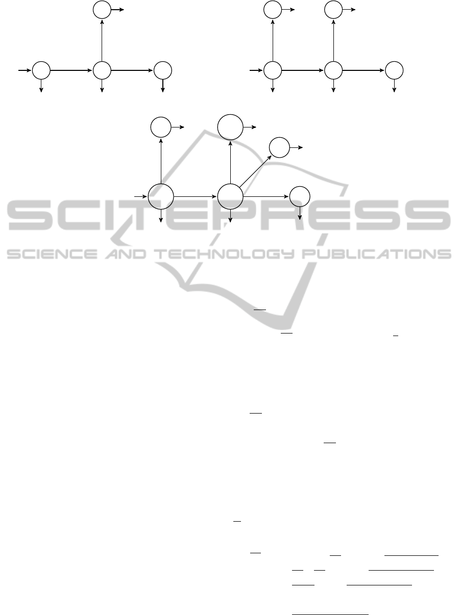
Proposition 4.5. Let A and B be two PWAs associ-
ated respectively with datasets X and Y . There exists
a PWA C for the dataset X ∪Y derived from A and B.
Proof. The idea is to construct the automaton C by
determinizing both automata A and B using the ac-
cessible subset-construction procedure. We give be-
low the definition of: R the set of states of the au-
tomaton C , and γ the function of final weights (the
functions µ and λ are obvious, and remain unchanged
as seen in Definition 4.3 and depicted in Figure 2),
and a mapping h from R to the set of states of P
X∪Y
,
which is the range of the polynomial P
X∪Y
.
Let A = (P,A
1
,µ
1
,λ
1
,γ
1
) be a PWA isomorphic, via
h
1
, to the automaton P
X
, and B = (Q, A
2
,µ
2
,λ
2
,γ
2
)
the one isomorphic, via h
2
, to the automaton P
Y
. We
define the PWA C = (R,A
1
∪ A
2
,µ,λ, γ) as follows
(p ∈ P and q ∈ Q):
• Set of states : R = {{p,q} | h
1
(p) = h
2
(q)} ∪
{{p} | h
1
(p) ∈ h
1
(P) \ h
2
(Q)} ∪ {{q} | h
2
(q) ∈
h
2
(Q) \ h
1
(P)},
• Final weights : γ({p,q}) = γ
1
(p) +
γ
2
(q);γ({p}) = γ
1
(p);γ({q}) = γ
2
(q).
The mapping h from R to range(P
X∪Y
) as follows :
h({p,q}) = h
1
(p); h({p}) = h
1
(p); h({q}) =
h
2
(q).
There is no difficulty to verify that the mapping h, as
defined above, is a weighted automata isomorphism
which is omitted here for space limitation.
In Figure 2, we illustrate the above construction by an
example of merging and determinizing of two simple
PWA associated with the following two datasets X =
{ab,ac},Y = {ac,ad,e}
4.2 Analysis of the Prefixial Weighted
Automata Merging Construction
The previous procedure, in Proposition 4.5, intro-
duces a construction method of a PWA associated
with a dataset. More interesting, it makes no as-
sumptions about the fragments X and Y , and there-
fore, it provides a flexible construction algorithm of
the union of two or more PWAs, either in batch or in-
cremental way.
Moreover, this construction offers some complexity-
related remarkable properties. Here, we mention
some of them.
The following lemma is induced from the inclusion-
exclusion principle.
Lemma 4.6. Let X and Y be two datasets. Then:
|P
X∪Y
| ≤ |P
X
| + |P
Y
| (4.3)
Consequently, we obtain this two corollaries about
the size of a PWA and the complexity of its construc-
tion.
Corollary 4.7. Let D be a dataset. Then:
|P
D
| ≤ |D| (4.4)
Likewise, and as the subset construction of a PWA
automaton associated with the dataset X ∪Y derived
from the PWAs associated with X and Y is guided by
the transitions of the smallest automaton, we can state
the following lemma.
Lemma 4.8. A PWA associated with the dataset X ∪Y
can be constructed from the PWAs associated with X
and Y in O(min(|P
X
|,|P
Y
|)) time.
DATA2015-4thInternationalConferenceonDataManagementTechnologiesandApplications
54

p
0
22
p
1
22
p
2
11
p
3
11
a/1 b/1
c/1
(a)
q
0
33
q
1
22
q
2
11
q
4
11
q
3
11
a/1
e/1
d/1
c/1
(b)
{p
0
,q
0
}
55
{p
1
,q
1
}
44
{p
2
}
11
{q
4
}
11
{q
2
}
11
{p
3
,q
3
}
22
a/1
e/1
b/1
c/1
d/1
(c)
Figure 2: two automata (a) and (b) and the merging one (c) by determinization.
Consequently, we can deduce the following
Proposition.
Proposition 4.9. Let D be a dataset. A PWA of D can
be constructed in O(|D|) time and space complexity.
Further, we can naturally generalize these results
to k datasets. This constitutes an important criterion,
that provides a fluid tuning and a flexible data parti-
tioning scheme, which is very useful in many aspects
of the problem. Indeed, it allows to deal with the
memory requirements, parallelization and/or incre-
mentality constraints, since, it does not matter, here,
the granularity of this partitioning: by transaction as
in (Cheung and Zaïane, 2003), or by batch as in (To-
tad et al., 2012), taking two or more data fragments.
The following corollary gives this extension.
Corollary 4.10. Let A
1
,.. .,A
k
be k PWA associated
respectively with the datasets X
1
,.. .,X
k
. One can
construct a PWA associated with the union X
1
∪ . .. ∪
X
k
in O(|X
1
| + ... + |X
k
|) time and space complexity.
4.3 Toward the Itemset Weighted
Automaton
The work done, so far, is a significant step toward
our objective. Recall that our goal is to construct
a weighted automaton that realizes the subsequence
polynomial S
D
associated with a dataset D. Let us de-
fine here another polynomial, which we refer to as the
prefixial-bar polynomial. The later serves as an inter-
mediate one, that guides us to obtain the targeted one
S
D
.
Definition 4.11. Let D be a dataset, and P
D
the asso-
ciated prefixial polynomial. The prefixial-bar polyno-
mial P
D
is:
P
D
= hP
D
,εi +
∑
u∈A
∗
a∈A
hP
D
,uaiua (4.5)
Obviously, the prefixial-bar polynomial of the
dataset D depends on the prefixial one. We give the
following proposition.
Proposition 4.12. Let D = {t
1
,.. .,t
n
} be a dataset.
Let P
D
and S
D
respectively the associated prefixial-
bar and the subsequence polynomials. Then:
P
D
= S
D
(4.6)
Proof. Let us start by checking that the Proposi-
tion 4.12 is true for one transaction t
i
taken from the
dataset D of n transactions.
So, let t
i
= a
i
1
a
i
2
... a
i
k
be a k-itemset. According to
the definitions in Sections 3 and 4, and the convention
a
i
= a
i
+ 1, we have:
P
t
i
= 1 + a
i
1
+ a
i
1
a
i
2
+ . .. + a
i
1
a
i
2
a
i
3
... a
i
k
So, P
t
i
= 1 + a
i
1
+ a
i
1
a
i
2
+ . .. + a
i
1
a
i
2
... a
i
k−1
a
i
k
= a
i
1
+ a
i
1
a
i
2
+ . .. + a
i
1
a
i
2
a
i
3
... a
i
k−1
a
i
k
= a
i
1
a
i
2
+ . .. + a
i
1
a
i
2
a
i
3
... a
i
k−1
a
i
k
...
= a
i
1
a
i
2
a
i
3
... a
i
k−1
a
i
k
= S
t
i
AUnifyingPolynomialModelforEfficientDiscoveryofFrequentItemsets
55

Now let us verify also the equality between the sum
of the prefixial-bar polynomials and the prefixial-bar
polynomial of the whole dataset D.
P
t
i
= hP
t
i
,εi +
∑
u∈A
∗
a∈A
hP
t
i
,uaiua
n
∑
i=1
P
t
i
=
n
∑
i=1
hP
t
i
,εi +
n
∑
i=1
∑
u∈A
∗
a∈A
hP
t
i
,uaiua
=
n
∑
i=1
hP
t
i
,εi +
∑
u∈A
∗
a∈A
n
∑
i=1
hP
t
i
,uaiua
= hP
D
,εi +
∑
u∈A
∗
a∈A
hP
D
,uaiua
= P
D
We’ve found that: P
t
i
= S
t
i
, so
n
∑
i=1
P
t
i
=
n
∑
i=1
S
t
i
which leads to P
D
= S
D
.
The construction of an automaton that compute the
dataset subsequence polynomial S
D
become now eas-
ier. Note that the polynomial P
D
can be rewritten to
show the link with the polynomial P
D
by adding null
terms:
P
D
= hP
D
,εi+
∑
u∈range(P
D
)
0×u+
∑
ua∈range(P
D
)
a∈A
hP
D
,uaiua
By bringing together the expressions of P
D
and that
of P
D
, we can note the bijection between each u in
P
D
and u in P
D
. Consequently, since u encodes the
subsequences of u (see Definition 3.1), it suffices,
thus, to add ε-transitions in paths labeled u in our au-
tomaton P
D
; However, we must be scrupulous about
coefficients, because adding ε-transitions may mul-
tiply the recognition paths of an itemset. This can
be fixed by state duplication. That is, for each state
u 6= ε, we create a second one (ua) with the right
coefficient (hP
D
,uai), the original becomes a non-
accepting state with null weight (0 × u). Notice that
this state/transition duplication is, here, artificial and
will be simulated as shown in Algorithm 3. This trick
also insures the values of the other terms in the rest of
the polynomial P
D
. We illustrate this idea by a simple
example of a dataset D containing only two transac-
tions D = {abc,ab}. In Figure 3, we give the two
automata: a PWA of D, and the extended one.
4.4 The Mining Algorithm
Once the PWA associated with D has been built us-
ing one of the processes introduced by the Proposi-
tion 4.5 or Corollary 4.10, it serves as a structure for
the problem space exploration. In our mining phase,
we explore the automaton using a depth-first traver-
sal as exhibited in Algorithm 2. The main strength
of our algorithm is that it doesn’t require any addi-
tional memory other than that needed for the WPA as
opposed to the previous approaches (see (Goethals,
2004)).
Algorithm 2: DISCOVER-FI(
S
,s,w,F ).
Require: a PWA of D, the support-threshold s, a set
of states Q
w
, and an itemset w
Ensure: The set of all FI
F ←
/
0  Initialization
for all a > w
|w|
do
(Q
wa
,hS
D
,wai) ← EXTEND(Q
w
,w,a)
if hS
D
,wai ≥ s then
F ← F ∪ {(wa,h
S
,wai)}
DISCOVER-FI(
S
,s,wa, F )
end if
end for
return F
Algorithm 3: EXTEND(Q
w
,w,a).
Require: set of states Q
w
, an itemset w, an item a
Ensure: The extended set of states Q
wa
P ← Q
w
R ←
/
0
while P 6=
/
0 do
q ← pick a state from P
if i(q) = a then
R ← R ∪ {q}
else if i(q) < a then
P ← P ∪ δ
+
(q)
end if
end while
return (R, γ(R))
The exploration begins with the invocation
DISCOVER-FI(s,{q
0
},ε,F ), where q
0
is the initial
state of the automaton. At each step, and starting
from the set of states Q
w
, an itemset w is extended by
concatenation with its successors by calling the func-
tion EXTEND(Q
w
,w,a). This call returns the set of
states Q
wa
of all paths labeled wa with their coeffi-
cients. The support of the concerned itemset wa is
then the sum of the coefficients of the elements in the
returned set Q
wa
, since γ(R) =
∑
r∈R
γ(r). If this ex-
tension succeeds with a frequent itemset, the process
will continue taking into account the last reached set
of states Q
wa
; Otherwise the returned couple is (
/
0,0).
Note that i(q) stands for the item-label of the transi-
tion leading to the state q, with i(q
0
) = ε, and δ
+
(q)
for the successor states of the state q.
DATA2015-4thInternationalConferenceonDataManagementTechnologiesandApplications
56

ε
22
a
22
ab
22
abc
11
a/1 b/1 c/1
(a)
ε
22
a
00
ab
00
abc
00
εa
22
ab
22
abc
11
a/1 b/1 c/1
b/1a/1 c/1
ε/1 ε/1 ε/1
(b)
Figure 3: a PWA (a) and its extended automaton (b).
Proposition 4.13. Algorithm 2 can be done in
O(
∑
w∈F
a>w
|w|
C
wa
) time and O(|Q|) space, where Q is the
set of states of the PWA, and F is the set of FI in the
dataset, and C
wa
is the time required to compute the
set Q
wa
by extending the set Q
w
.
Proof. Our automaton is acyclic over a sorted alpha-
bet. So, the length of any path is upperbounded by
|Q|. C
wa
is the time needed to the call of the function
EXTEND, which computes the set Q
wa
taking into ac-
count the last obtained set of states Q
w
. Let, with-
out loss of generality, C
wa
= |Q
wa
|, hence for each
itemset w = w
1
... w
k
in F , we have: C
w
1
+C
w
1
w
2
+
... +C
w
1
w
2
...w
k
< |Q|. Consequently, if F
M
denote the
set of maximal frequent itemsets, and F
L
the set of
maximal frequent itemsets w.r.t to the prefixial re-
lation (F
M
⊆ F
L
⊆ F ), we obtain the inequality :
|F
M
||Q| ≤
∑
w∈F
C
wa
≤ |F
L
||Q| ≤ |F ||Q| ≤ |F ||D|.
Further, the memory requirement of the recursive ex-
ploration is also upperbounded by |Q|; it does not
matter the length of the itemset to be recognized or
the current level of the exploration, since the returned
sets, during the traversal, are pairwise disjoint and
their union is Q in the worst case.
5 COMPARISON AND
UNIFICATION
A theoretical framework based on formal concept
analysis and lattice theory is presented early in (Godin
et al., 1995; Zaki and Ogihara, 1998). Recently, in
(Pijls and Kosters, 2010) attempt is made to unify the
common FI-algorithms w.r.t the traversal paradigms
well-known in the operations research community.
Our model uses formal series, which are mappings
between a monoid M and a semiring K. The appropri-
ate choice of M and K, and the automaton characteris-
tics which realizes it is driven by the targeted applica-
tion and needed performances. For the basic version
of the FI-mining problem, that is mining itemsets,
we opted for the counting semiring (N,+,×,0,1) be-
cause it offers an intuitive and easy implementation.
We are convinced that this framework can be gen-
eralized for mining other elaborated items such as se-
quences, trees or graphs, provided that much more
work must be carried out to define monoids of these
elements with the appropriate operations and the cor-
responding implementations by means of specific au-
tomata.
In what follows, we compare our model against
the main state of the art techniques, and explain how
these ones can be derived from it.
Level-wise Approaches. An Apriori-like algo-
rithm (Agrawal and Srikant, 1994) proceeds level by
level. First, it computes the frequent singletons and
then forms from these a set of candidate doublets. Af-
ter determining the frequent doublets, it continues to
generate the set of frequent triplets and so on, until no
new frequent itemsets can be generated. Despite its
limits: generating a huge number of candidates and
repetitive database scans, this algorithm stay one of
the top cited algorithms in the DM community (Wu
et al., 2008). Our model can be modified to fit a sim-
ilar principle if we use an adapted deterministic ver-
sion of the defined automaton, and perform a simple
linear traversal of it in a stepwise fashion. Notice that
this adaptation to Apriori allows to devise a more ef-
ficient algorithm, since in one hand any itemset have
only a unique acceptation path, and in the other hand
we do not make use of candidate generation neither
database scans for support computation.
Vertical Approaches. The main benefit of the verti-
cal approach (Zaki, 2000) against the level-wise ap-
proaches is speedy in the support calculation via set
intersections. However, the drawback as mentioned
AUnifyingPolynomialModelforEfficientDiscoveryofFrequentItemsets
57

in the introduction and by the author itself in an im-
proved version is when the intermediate results be-
come too big. Our method, in contrast, is based on a
simple output weight read or their summation without
need of any additional memory.
The vertical approach can be seen as a formal se-
ries on the powerset semiring of the set T of trans-
actions (2
T
,∪,∩,
/
0,T ), with the min operation com-
puted by set intersection, and the sum by the union.
The weight of a transition represents the cardinality
of the tidlist of the itemset formed by the path from
the root
/
0 to the considered node.
FPGrowth Approaches. It seems to the first glance
that our defined automaton is an FPTree (Han et al.,
2000) by an other way. We must emphasize at the
outset that the similarity to FPTree or other concepts
in any of the previous work should be seen as a posi-
tive point and not the inverse, since our purpose is the
definition of a unifying model. We claim, in the other
hand, that this is not correct enough. First of all, our
automaton is not a data structure but rather a computa-
tional model, which can be implemented in different
ways. Secondly, The mining algorithms are signifi-
cantly different. While FPGrowth use a heavily in-
termediate memory, and also time overhead, for con-
ditional databases and conditional FPTrees construc-
tion, our model do not require any additional mem-
ory other that necessary for the automaton. Further,
and unlike FPGrowth, the open ordering adopted in
our model leads to significant time improvement both
in the construction phase (only one scan is required),
and the mining one, since there is no need to repetitive
resorting, neither database projections. Additionally,
we argue that our approach outperforms also exten-
sion of FPTrees like CATSTree (Cheung and Zaïane,
2003), which the building may require many node
swaps to maintain its integrity (the support of a par-
ent must be greater than the sum of its children’s sup-
ports), and incurs consequently some overhead. To
the end of unification, we can view these approaches
as a sequence of right derivations by the set of items
A of our dataset subsequence polynomial S
D
, or like
the exploration of the mirror of the automaton. In-
deed, the right derivative of the polynomial S
D
w.r.t
an item a produces the polynomial representation of
the a-conditional database in FPGrowth.
Tropical Semiring. An equivalent modeling to our
approach can be obtained by using the tropical semir-
ing, computed by a different weighted automaton,
where the transitions carry the output weights. In
this case, the output weights of all states are ∞. The
weight of a path is the minimum of the weights of
its transitions. It is obvious to note that this model,
although equivalent, is expensive compared to which
we have adopted, that consists to a simple read of the
state output weight.
6 CONCLUSION
We have proposed a new model for mining FI. This
model is based on formal series over the semiring
(N,+,×, 0,1), whose the range constitutes the item-
sets and the coefficients their supports. We argue that
the strength of the introduced formalism are numer-
ous. First, while remaining simple and intuitive, it
is complete to model the basic problem. Secondly,
it allows the decomposition of the problem to deal,
eventually, with the constraints of time or space or
both, into independent sub-problems which leads to
parallelization and/or incrementatlization processes.
Furthermore, the proposed model can be generalized
to handle more complex items such as sequences,
trees...etc. On the practical side, the model provides
an implementation whose performance are proved to
be competitive.
We have also, reduced this problem, in its ba-
sic version, to that of word recognition, allowing an
implementation without extra memory in O(|F
L
||Q|)
time and O(|Q|) space.
In future work, we can improve the mining al-
gorithm by avoiding to recompute the extensions for
itemsets u and v having the same returned set of states
after the call to the function EXTEND (Q
u
= Q
v
). This
can be done by working on the deterministic automa-
ton equivalent to S
D
. We will show, in a subsequent
work, that this optimization gives also a new time up-
perbound, which is the number of states of this deter-
ministic automaton, which we conjecture will not be
exponential. Furthermore, despite that it is not trivial,
it would be very interesting to study other properties
of the defined automaton such as its minimization.
We also plan to extend this approach to mine, first,
the set of frequent maximal and closed itemsets, and
then sequences and trees. Finally, the algebraic as-
pects of formal series deserves more investigation,
and might lead to other theoretical or practical results.
REFERENCES
Agrawal, R. and Srikant, R. (1994). Fast algorithms
for mining association rules in large databases. In
VLDB’94, Proceedings of 20th International Confer-
ence on Very Large Data Bases, September 12-15,
1994, Santiago de Chile, Chile, pages 487–499.
Cheung, W. and Zaïane, O. R. (2003). Incremental min-
ing of frequent patterns without candidate generation
DATA2015-4thInternationalConferenceonDataManagementTechnologiesandApplications
58

or support constraint. In 7th International Database
Engineering and Applications Symposium (IDEAS
2003), 16-18 July 2003, Hong Kong, China, pages
111–116.
Godin, R., Missaoui, R., and Alaoui, H. (1995). Incremen-
tal concept formation algorithms based on galois (con-
cept) lattices. Computational Intelligence, 11:246–
267.
Goethals, B. (2004). Memory issues in frequent itemset
mining. In Proceedings of the 2004 ACM Symposium
on Applied Computing (SAC), Nicosia, Cyprus, March
14-17, 2004, pages 530–534.
Goethals, B. and Zaki, M. J., editors (2003). FIMI ’03,
Frequent Itemset Mining Implementations, Proceed-
ings of the ICDM 2003 Workshop on Frequent Item-
set Mining Implementations, 19 December 2003, Mel-
bourne, Florida, USA, volume 90 of CEUR Workshop
Proceedings. CEUR-WS.org.
Han, J., Cheng, H., Xin, D., and Yan, X. (2007). Frequent
pattern mining: Current status and future directions.
Data Min. Knowl. Discov., 15(1):55–86.
Han, J., Pei, J., and Yin, Y. (2000). Mining frequent pat-
terns without candidate generation. In Proceedings
of the 2000 ACM SIGMOD International Conference
on Management of Data, May 16-18, 2000, Dallas,
Texas, USA., pages 1–12.
Han, J., Pei, J., Yin, Y., and Mao, R. (2004). Min-
ing frequent patterns without candidate generation: A
frequent-pattern tree approach. Data Min. Knowl. Dis-
cov., 8(1):53–87.
Hipp, J., Güntzer, U., and Nakhaeizadeh, G. (2000). Algo-
rithms for association rule mining - A general survey
and comparison. SIGKDD Explorations, 2(1):58–64.
Pasquier, N., Bastide, Y., Taouil, R., and Lakhal, L. (1999).
Discovering frequent closed itemsets for association
rules. In Proceedings of the 7th International Confer-
ence on Database Theory, ICDT ’99, pages 398–416,
London, UK, UK. Springer-Verlag.
Pijls, W. and Kosters, W. A. (2010). Mining frequent item-
sets: a perspective from operations research. Statistica
Neerlandica, 64(4):367–387.
Salomaa, A., Soittola, M., Bauer, F., and Gries, D. (1978).
Automata-theoretic aspects of formal power series.
Texts and monographs in computer science. Springer-
Verlag.
Totad, S. G., Geeta, R. B., and Reddy, P. V. G. D. P.
(2012). Batch incremental processing for fp-tree con-
struction using fp-growth algorithm. Knowl. Inf. Syst.,
33(2):475–490.
Valtchev, P., Missaoui, R., and Godin, R. (2008). A frame-
work for incremental generation of closed itemsets.
Discrete Applied Mathematics, 156(6):924–949.
Wille, R. (1982). Restructuring lattice theory: An approach
based on hierarchies of concepts. In Rival, I., editor,
Ordered Sets, volume 83 of NATO Advanced Study In-
stitutes Series, pages 445–470. Springer Netherlands.
Wu, X., Kumar, V., Quinlan, J. R., Ghosh, J., Yang, Q., Mo-
toda, H., McLachlan, G. J., Ng, A. F. M., Liu, B., Yu,
P. S., Zhou, Z., Steinbach, M., Hand, D. J., and Stein-
berg, D. (2008). Top 10 algorithms in data mining.
Knowl. Inf. Syst., 14(1):1–37.
Yang, Q. and Wu, X. (2006). 10 challenging problems in
data mining research. International Journal of Infor-
mation Technology and Decision Making, 5(4):597–
604.
Zaki, M. (2000). Scalable algorithms for association min-
ing. Knowledge and Data Engineering, IEEE Trans-
actions on, 12(3):372–390.
Zaki, M. J. and Ogihara, M. (1998). Theoretical foundations
of association rules. In 3rd ACM SIGMOD Workshop
on Research Issues in Data Mining and Knowledge
Discovery.
Zaki, M. J. and Wagner Meira, J. (2014). Data Min-
ing and Analysis: Fundamental Concepts and Algo-
rithms. Cambridge University Press.
AUnifyingPolynomialModelforEfficientDiscoveryofFrequentItemsets
59