A Proposal based on Frequency Response for Multi-Model
Controllers
Anderson Luiz de Oliveira Cavalcanti
Federal University of Rio Grande do Norte, Natal, RN, Brazil
Keywords: MPC, Multi Model Control.
Abstract: This paper presents an alternative approach to control nonlinear plants. The nonlinear system to be
controlled is decomposed into a number of operating points and a GPC controller is properly designed,
based on local linear model for each point. A metric based on frequency response of each local linear model
is proposed in order to consider the contribution of each local controller in the signal sent to the plant. Two
applications are presented. The first application in a simulated plant consists of a continuous stirred tank
reactor (CSTR) and the second consists of a coupled tanks system level control.
1 INTRODUCTION
In the industry are found processes that work in
large operating ranges. Batch processes (Foss et al.,
1995), as chemical reactors, are classic examples of
this type of process. The main solution in these cases
would be to obtain a non-linear complex model,
requiring, in the case of using predictive controllers,
the use of nonlinear prediction and optimization,
which is not a trivial task (Camacho and Bordons,
1999).
In order to provide a simpler solution for the
problems mentioned above, a known approach, in
academia, as multi-models approach has been
investigated (Boling et al., 2007), (Dougherty and
Cooper, 2003a), (Dougherty and Cooper, 2003b),
(Arslan et al., 2004) and (Normey- Bravo and Rich,
2009). This approach seeks to decompose the
process range of operating at various operating
points usual in the same place and obtain a valid
model for each of these points. A validation
function, called a metric is defined to indicate what
is the most appropriate model at a given moment of
sampling. Such a metric is used to calculate
weighting factors, the application of which will be
described below. There are basically two types of
multi-model approaches, which will be detailed
below also.
The first approach uses the weighting factors to
compute a global model formed by the convex
combination of local models obtained and a single
controller is designed from said master (Foss et al.,
1995) (Azimadeh et al., 1998) (Dumitrache and
Constantine, 2000) (Pickhardt, 2000) and
(Cavalcanti et al., 2007a).
The second type of approach designs a suitable
controller for each model of each operating point. In
this case, the control signal to the process is a
convex combination of the computed control signals
(Cavalcanti et al., 2007b), (Cavalcanti et al., 2008),
(Arslan et al., 2004), (Wen et al., 2006), (Dougherty
and Cooper, 2003) and (Dougherty and Cooper,
2003b).
This article is based on the second type of
approach mentioned. Most existing literature are
based on the metrics or statistics of the process (Foss
et al., 1995) or standards (Dougherty and Cooper,
2003) (Dougherty and Cooper, 2003b), (Arslan et
al., 2004) (Cavalcanti et al., 2007b) and (Cavalcanti
et al., 2008). This work, in particular, consider the
frequency response of each local model compared to
the frequency response of each current approximate
model obtained by interpolation at each sampling
instant.
The choice of use of a predictive controller based
on the highlight that this is gaining in terms of
industrial applications (García, Prett and Morari,
1989). This highlight is observed as the same, and
can be applied in a wide range of processes,
including processes with long delays and non-
minimum phase, you can easily incorporate the
constraint treatment in the problem formulation
(Camacho and Bordons 1999).
223
Luiz de Oliveira Cavalcanti A..
A Proposal based on Frequency Response for Multi-Model Controllers.
DOI: 10.5220/0005546202230229
In Proceedings of the 12th International Conference on Informatics in Control, Automation and Robotics (ICINCO-2015), pages 223-229
ISBN: 978-989-758-122-9
Copyright
c
 2015 SCITEPRESS (Science and Technology Publications, Lda.)

This article is organized as follows: section 2
shows the theoretical formalization of multi-model
approach used in this work; Section 3 shows the
metric based on frequency response proposal;
Section 4 shows the application results in a
simulated continuous stirred tank reactor and in a
real system level control, as well as discussions on
them. Section 5 provides the conclusions.
2 THEORETICAL
FORMALIZATION OF
MULTI-MODEL APPROACHES
Consider a nonlinear system with multiple operating
points, which is segmented into a set Φ containing
NPO operating regimes. Each operating regime is
defined as a subset Φ
i
⊂ Φ with i = 1,..,NPO. An
operating point is typically denoted by a function φ
represented by a subset of input and output like
φ =
H(y, u). It is assumed that there is a metric ρ
i
: Φ 
[0,1], which is designed so that its value is close to
one for operating points where the local model i is a
good description of the system and close to zero
otherwise. If the system’s operating range is broken
down into NPO operating systems, so that
Φ
1
,…,Φ
NPO
⊂ Φ, then for each local model is
defined a particular metric ρ
i
( φ ) with i = 1,…, NPO.
For each operating system, a model of discrete
transfer function type can be described:
y(z) =
G
i
(z)u(z)
(1)
where G
i
(z), u(z) and y(z) are the transfer function of
the process valid for the operating point i, the
deviation of the process input and the deviation of
the process output. For each operating point, a
controller is designed, and its output at time k is
denoted by u
i
(k). The control action effectively sent
to the process is given by:
u(k) = u
i
(k)w
i
( φ )
i=1
NPO

(2)
where u (k) is the control signal computed by the
i-th controller and w
i
(φ) is the weighting factor
assigned to that controller given by:
w
i
( φ ) =
ρ
i
(
φ
)
ρ
j
( φ )
j =1
NPO

(3)
The following property to (3) is defined to ensure
the convexity:
w
i
( φ )
i=1
NPO

=1
(4)
This paper, specifically, the controller designed
for each operating point is a Generalized Predictive
Control (GPC) (Clarke et al., 1987). The considered
tunning parameters are the prediction horizon (NY),
the control horizon (NU) and the weighting of the
control signal (λ). More details on the GPC can be
obtained from (Clarke et al., 1987).
3 METRIC BASED ON
FREQUENCY RESPONSE
3.1 The Proposed Metric
The methodology proposed in this work takes into
account the difference in dynamics between the
transfer functions, appointed by the different
frequency responses. It is assumed that, for all
operating points, a linear model of the process can
be obtained. At each sampling time, an estimation of
the parameters change, based on interpolation, is
made considering the current output y(k) (current
model). The current model is compared, in terms of
frequency response, with the determined models in
operating points. An index called dynamic measure
(MD) sistem, is defined. The dynamic measure
(MD) is given by the area under the frequency
response curve corresponding to the module. Thus,
for each local model of each operating point defined
the MD is calculated as follow:
0
() (),1,...,
N
jh jh
ii
M
De Ge d i NPO
ω
ωω
ω ==

(5)
where h is the sampling time and ω
N
is the Nyquist
Frequency.
The function that describes the system’s metric,
according to the criteria established in section 2, is
given by:
()()
() ()
max ( ) min ( )
( ) , 1,...,
jh jh
ii
i
jh jh
ia
MD e MD e
iNPO
MD e MD e
ωω
ωω
ρϕ
−
==
−
(6)
where MD
a
(e
j ω h
) is the dynamic measure of the
system uat the current sampling time k. Thus,
considering the metric, the proposed control
algorithm is described as follows:
Step 1: Read the output of the process at time k,
y(k);
ICINCO2015-12thInternationalConferenceonInformaticsinControl,AutomationandRobotics
224

Step 2: Calculate the estimated G
a
(z) by
interpolation based on y (k);
Step 3: Compute the value (MD
a
(e
j ω h
)) based on
G
a
(z);
Step 4: Compute the values of ρ
i
(φ), i = 1, …, NPO;
Step 5: Compute the values of the weights of the
local controllers w
i
(φ), i = 1, …, NPO;
Step 6: Compute the control signal by convex
combining of each local controller signal - see
equation (2);
Step 7: Apply the control signal in the plant;
Step 8: Wait for the next sampling period h and
return to Step 1.
Note that the calculation of integral in (9) is
computed numerically.
4 RESULTS AND DISCUSSIONS
4.1 Application Example 1: Simulated
Continuous Stirred Tank Reactor
(CSTR)
The plant to be controlled, in this simulated case,
consists of a continuous stirring tank reactor which
is a process widely found in Chemical and
Biochemical Engineering. Normally, to irreversible
exothermic reactions, adiabatic mode reagents leads
to large production rates, so in order to maintain the
temperature within a certain range, the generated
heat has to be removed by cooling. The vessel is
assumed to be perfectly mixed, and a single
irreversible reaction exothermic first order occurs.
Thus, the variable to be controlled is the temperature
of the reactor and the manipulated variable is the
cooling temperature.
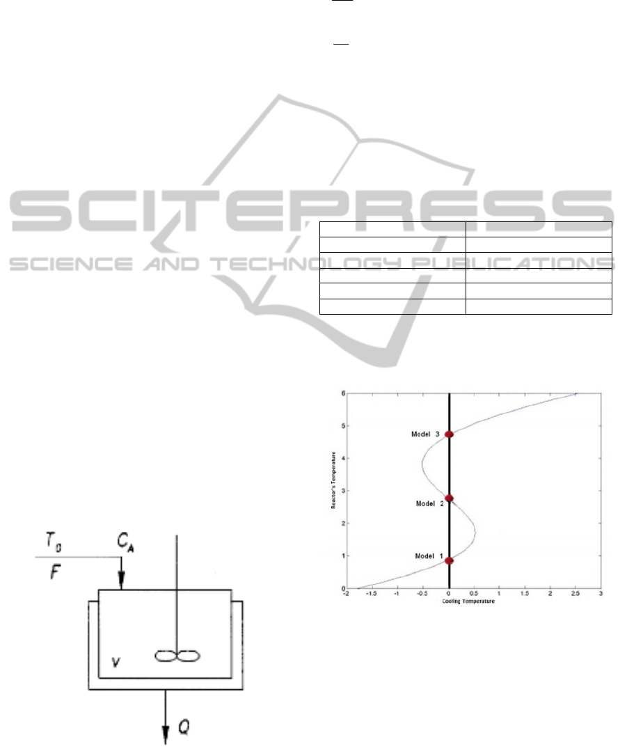
Figure 1 shows an illustration of this reactor:
Figure 1: Continuous Stirred Tank Reactor.
A nonlinear space state model to the reactor is
found in Arslan et al. (2004) and Uppal, et al.
(1976). The model is based on mass and energy
balance of the tank as shown below:
(1 ) exp( / (1 / )) ( 1)
A
Aa A f
dC
CD C T T C
dt
γ =− + − + − −
(7)
(1 ) exp( / (1 / )) ( )
aA R
dT
TBD C T T T T
dt
γβ =+⋅ − + − −
(8)
where C
A
is the concentration of product of the
reactor given in gmol/L, T is the temperature of the
reactor (controlled variable) given in Kelvin, T
R
is
the cooling temperature (manipulated variable)
given in Kelvin and C
f
is the reactor feed
concentration given in gmol/L. Typical values of the
constants shown in (7) and (8) are shown in Table 1.
Table 1: Parameters of the CSTR nonlinear model.
Constant Value
Da 0.072
γ
20
B 8
β
0.3
Cf 1
Figure 2 shows the curve of the steady state system.
Here, we consider three operating points, as shown
in curve for T
R
= 0.
Figure 2: Steady State curve to Continuous Stirred Tank
Reactor model.
For T
R
= 0, we see, in Figure 4, three equilibrium
points, which will be considered as the operating
points in this work. Linearizing the model (7) and
(8) around the equilibrium points and discretizing
them to h = 0.1 minutes, we obtain the following
models:
AProposalbasedonFrequencyResponseforMulti-ModelControllers
225

1
2
0.02964 0.02638
()
1.865 0.8694
z
Gz
zz
−
=
−+
(9)
2
2
0.03211 0.0269
()
1.969 0.9646
z
Gz
zz
−
=
−+
(10)
3
2
0.03362 0.02199
()
1.837 0.8521
z
Gz
zz
−
=
−+
(11)
For each of these models, a GPC was tuned, to
the given operating point, considering a maximum
settling time of 5 minutes. The tuning parameters of
each local controller are shown in Table 2. For
comparison, the proposed method is compared with
a single-model GPC using the model 3 shown in
(11) and the method proposed in Arslan et al.
(2004).
Table 2: Tuning parameters of the local GPC controller in
CSTR example.
Operating Point
λ
NY=NU
Point 1 3 15
Point 2 2 15
Point 3 1 20
The objective of controllers, in this example, is
to track the references as shown in Figure 3. The
references considered is the operating point.
Figure 3: Process output (Cooling temperature).
Analysing the Figure 3, we observe a better
performance of the multi-modelo controller,
compared with the other controllers, in terms of less
overshoot and shorter stabilization, particularly
when the process is far from the third operating
point. When the process is close to the third
operating point, this improvement is not as
significant, since the multi-model is replaced as the
dominant controller the controller designed for that.
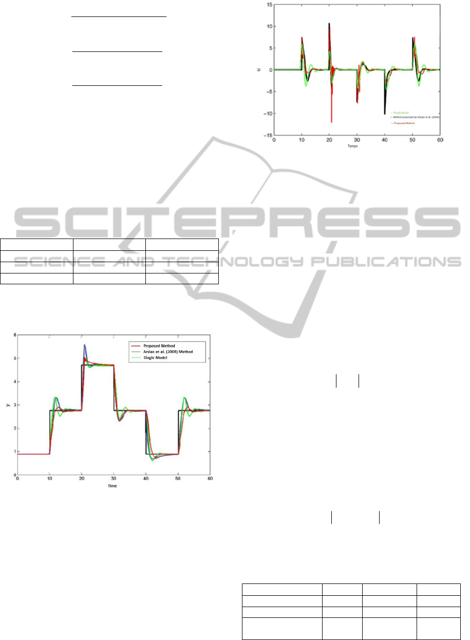
Figure 4 shows the control signal for this simulation.
Figure 4: Control Signal.
The authors of Arslan et al. (2004) consider a
metric known as Gap Metric that is based in H
∞
norm. In Arslan et al. (2004), the designed
controllers are Proportional-Integral (PI). However,
this comparison is possible because the design
criteria used for each controller in this work are the
same, that is, each controller is designed so as to
obtain maximum settling time of 5 minutes.
The control effort generated by the multi-model
scheme is shown in Figure 6, most of the time, less
than the control effort single-model schema.
For a better analysis of the performance of
controllers, some classic indices of control literature
are compared. In (Goodhart, et al., 1994) the authors
present some indices that assess the controller
performance. The first index is given by:
€
ε
1
= u(k) /N

(12)
where N is the number of control signals applied to
the process so that it achieves the desired response.
The content presented in (12) represents the energy
used by the process to achieve the desired response.
The variance of the actuators is given by:
2
21
(() )/uk N εε =−

(13)
The process output deviation in terms of the integral
of absolute error (IAE) is:
3
() ()/rk yk N ε =−

(14)
Table 3 shows the indexes considered for the three
simulations.
Table 3: Performance indexes for the CSTR example.
Controller
ε
1
ε
2
ε
3
Single model 0.678 2.523 0.164
Proposed Method 0.506 1.931 0.152
Method proposed in
Arslan et al. (2004)
0.613 0.613 0.613
ICINCO2015-12thInternationalConferenceonInformaticsinControl,AutomationandRobotics
226

Quantitative analysis shows, according to the
figures, that proposal in this paper provides less
energy spent by the process, the lower variance of
actuators and lower tracking error when compared to
the other controllers.
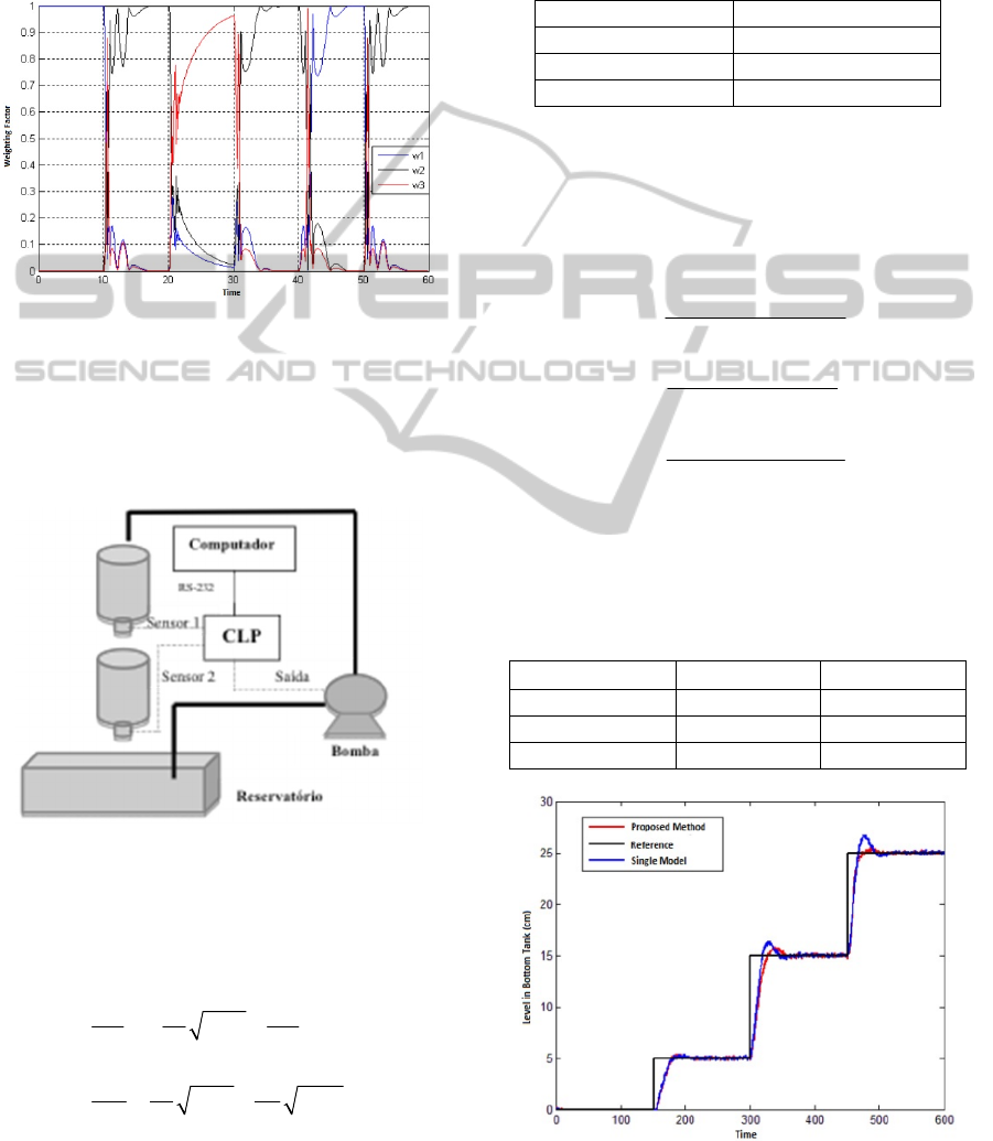
The variations in the weights of the three controllers
as function of time are shown in Figure 5.
Figure 5: Weights of the controllers.
4.2 Application Example 2:
Level Control in Coupled Tank
The second application of this work is on a real
system of coupled tanks (Figure 6).
Figure 6: Coupled tanks system.
Considering L
1
, L
2
and V
p
as the top tank level in
cm, the bottom tank level in cm and the pump
voltage in volts, respectively, the following
equations describe the states of the system:
11
1
11
2
m
p
K
dL a
gL V
dt A A
=− +
(15)
21 2
12
12
22
dL a a
gL gL
dt A A
=−
(16)
where a
1
and a
2
are the areas of the outlet holes of
lower tank and the upper tanks respectively, A
1
and
A
2
are the areas of the cross sections of the upper
and lower tanks respectively, K
m
is the constant of
the pump, and g = 981 cm/s
2
is the gravitational
acceleration. The values of the constants used for
testing in this study are described in Table 4.
Table 4: Parameters of the coupled tanks model.
Parameters Values
A
1
and A
2
15.518 cm
2
a
1
and a
2
0.1781 cm
2
K
m
4.6 (cm
3
/s).V
In this application the controlled variable is the
level of the bottom tank and the manipulated
variable is the voltage in the pump. In this case are
also considered three operating points. Linearizing
the model for 10cm, 15cm and 20cm, we obtain the
following discrete models for h = 0.5s:
1
2
0.004057 0.003906
()
1.889 0.8925
z
Gz
zz
−
=
−+
(17)
2
2
0.00238 0.002328
()
1.935 0.9365
z
Gz
zz
−
=
−+
(18)
3
2
0.001852 0.001821
()
1.95 0.9504
z
Gz
zz
−
=
−+
(19)
The tuning parameters in this case, shown in
Table 5, were obtained trying to get a settling time
of less than 50s.
Table 5: Tuning parameters of the local GPC controller in
coupled tanks example.
Operating Point
λ
NY=NU
Point 1 85 15
Point 2 75 15
Point 3 65 15
Figure 7: Controlled level in bottom tank (in cm).
AProposalbasedonFrequencyResponseforMulti-ModelControllers
227

In this application, we compare the proposed
controller with the single-model controller using the
model in operating point 1. The results are shown in
Figure 7. In the experiment, the system starts with
empty tanks. In a given time (time = 150 s.)
Reference is changed to the first operating point.
Then (time = 300 s), the reference to the controllers
is switched to the second operating point, and just
after (time = 450 s.) for the third operating point.
Similarly to the reactor of example, when the
system diverges from the first operating point, the
multi-controller model has better performance.
Figure 8 shows the control signals applied to the
pump, in volts, for the two trials. Note that in neither
case the input constraints (maximum voltage of 22V
pump) were violated because the system did not
operate near its constraint region. As the designed
GPCs controllers are subject to constraint on plant
input, the convex combination of the output of each
controller also produce a control signal within the
constraint limits.
Figure 8: Control signal – voltage in the pump (in volt).
Figure 9 shows the variation in weights of the
controllers as function of time.
Figure 9: Weights of the controllers.
Also for this application example, to quantitatively
evaluate the comparison made, the indexes showed
in (12), (13) and (14) are considered. Table 6 shows
the indexes to the present case.
Table 6: Performance indexes for the CSTR example.
Controller
ε
1
ε
2
ε
3
Single model 4.78 11.15 6.45
Proposed Method 4.46 11.01 6.34
We can see, for the evaluation of Table 6, the
proposed controller compared to the single model
controller has better performance.
5 CONCLUSIONS
Was presented in this paper an alternative approach
to nonlinear predictive control. The multi-model
approach has become an attractive alternative
proposal, because it uses the whole theoretical
framework of linear controller, which is quite
consolidated in academia, to control with results, in
many cases, better, as demonstrated this work and
the works here referenced.
The metric proposed here reflects well the
process change the operating point, pondering
consistently the isolated controllers designed.
The results shown in this work, both in
simulation in a physical plant, revealed an
improvement, properly evaluated by indexes,
compared to controllers with single model.
REFERENCES
Arslan, E., Çarmurdan, M., Palazoglu, A. e Arkun, Y.
(2004). Multi-Model Scheduling Control of Nonlinear
Systems Using Gap Metric, Ind. Eng. Chem. Res., vol.
43, pp 8275-8283.
Azimadeh, F., Palizban, H. A. e Romagnoli, J.A. (1998).
On Line Optimal Control of a Batch Fermentation
Process Using Multiple Model Approach, Proceedings
of the 37th IEEE Conference on Decision and Control,
pp. 455- 460.
Böling, J. M, Seborg, D. E e Hespanha, J. P. (2007).
Multi- model adaptive control of a simulated pH
neutralization process, Control Eng. Practice, vol. 15,
pp. 663-672.
Bravo, C. O. A. e Normey-Rico, J. E. (2009). Controle de
Plantas Não Lineares Utilizando Controle Preditivo
Linear Baseado em Modelos Locais, Revista Controle
and Automação, Vol. 20, n. 4, pp. 465-481.
Camacho, E. F. e Bordons, C. (2003). Model Predictive
Controle, Springer-Verlag, New York.
ICINCO2015-12thInternationalConferenceonInformaticsinControl,AutomationandRobotics
228

Cavalcanti, A. L. O, Fontes, A. B. e Maitelli, A. L.
(2007a). A Multi-Model Approach For Bilinear
Generalized Predictive Control. Proceedings of 4th
International Conference on Informatics in Control,
Automation and Robotics, pp. 289-295, Angers.
Cavalcanti, A. L. O, Fontes, A. B. e Maitelli, A. L.
(2007b). eneralized Predictive Control Based in
Multivariable Bilinear Multimodel. Proceedings of 8th
International IFAC Symposium on Dynamics and
Control of Process Systems, pp. 91-96, Cancun.
Cavalcanti, A. L. O, Fontes, A. B. e Maitelli, A. L. (2008).
Uma Abordagem com Múltiplos Modelos Para o
Controlador Preditivo Generalizado Bilinear
Multivariável Com Compensação Iterativa. Anais do
XVII Congresso Brasileiro de Automática, Juiz de
Fora/MG.
Clarke, D.W., Mohtadi, C. e Tuffs, P.S. (1987).
Generalized Predictive Control Parts 1 and 2,
Automatica, vol. 21, n. 2.
Constantin, N. e Dumitrache, I. (2002). Robust Control of
Nonlinear Process Using Multiple Models,
Proceedings of 15th IFAC World Congress, pp. 365-
370, Barcelona.
Dougherty, D. e Cooper, D. (2003a). A Practical Multiple
Model Adaptive Strategy for Single-Loop MPC,
Control Engineering Pratice, vol. 11, pp. 141-159.
Dougherty, D. e Cooper, D. (2003b). A Practical Multiple
Model Adaptive Strategy for multivariable MPC,
Control Engineering Pratice, vol. 11, pp. 649-664.
Foss, B.A., Johansen, T.A. e Sorensen, A.V
(1995).Nonlinear Predictive Control Using Local
Models Applied to a Batch Fermentation Process.
Control Eng. Practice, pp. 389-396.
Goodhart, S. G., Burnham, K. J. e James, D.J.G. (1994).
Bilinear Self-tuning Control of a high temperature
Heat Treatment Plant. IEEE Control Theory Appl.:
Vol. 141, no 1, pp. 779-783.
Morari, M., Garcia, C.E. e Prett, D. M. (1989). Model
predictive control: Theory and practice A survey,
Automatica, vol. 25, n 3, pp. 335-348.
Pickhardt, R. (2000). Adaptive Control of a Solar Power
Plant Using a Multi-Model, IEE Proc.-Control Theory
Appl., vol. 47, n. 5, pp 493-500.
Uppal, A., Ray, W. H. e Poore, A. B. (1974) On the
Dynamic Behavior of Continuous Stirred Tank
Reactors, Chem. Eng. Sci., 29, 967-977.
Wen, T., Caifen, F. e Liu, J. (2006). Mult-Model Control
of a Boiler-Turbine Unit, Proceedings of China
Control Conference, pp. 200-204.
AProposalbasedonFrequencyResponseforMulti-ModelControllers
229