Off-line State-dependent Parameter Models Identiﬁcation using Simple

Fixed Interval Smoothing

Elvis Omar Jara Alegria, Hugo Tanzarella Teixeira and Celso Pascoli Bottura

Semiconductors, Instruments, and Photonics Department, School of Electrical and Computer Engineering,

State University of Campinas - UNICAMP, Av. Albert Einstein, N. 400 - LE31 - CEP 13081-970, Sao Paulo, Brazil

Keywords:

Time Series Identiﬁcation, State-dependent Parameter, Data Reordering.

Abstract:

This paper shows a detailed study about the Young’s algorithm for parameter estimation on ARX-SDP models

and proposes some improvements. To reduce the high entropy of the unknown parameters, data reordering

according to a state ascendant ordering is used on that algorithm. After the Young’s temporal reordering

process, the old data do not necessarily continue so. We propose to reconsider the forgetting factor, internally

used in the exponential window past, as a ﬁxed and small value. This proposal improves the estimation

results, especially in the low data density regions, and improves the algorithm velocity as experimentally

shown. Other interesting improvement of our proposal is characterized by the ﬂexibility to the changes on the

state-parameter dependency. This is important in a future On-Line version. Interesting features of the SDP

estimation algorithm for the case of ARX-SDP models with unitary regressors and the case with correlated

state-parameter are also studied. Finally a example shows our results using the INCA toolbox we developed

for our proposal.

1 INTRODUCTION

Parameters of linear regression models can be satis-

factorily estimated by using conventional estimation

methods for Time Variable Parameters (TVP) based

on least squares techniques, but its time parameter

variations must be slow compared to the system state

variations (Yaakov Bar-Shalom, 2001). But when the

system presents State Dependent Parameters (SDP)

(Priestley, 1988) the model response can be heavily

nonlinear and even chaotic. The regression models

with SDP, called SD-ARX (Priestley, 1988; Young

et al., 2001) or quasi-ARX (Hu et al., 2001; F. Pre-

vidi, 2003), are always non-linear due to the product

between the regressor function and the SDP. Conven-

tional methods can’t estimate SDP models because

parameters vary very fast.

Young proposed a solution to SDP estimation

(Young et al., 2001). It’s based in a special tempo-

ral data reordering to smoothen the parameter varia-

tions. This proposed algorithm uses an optimal Fixed

Interval Smoothing (FIS) algorithm as a ﬁrst approx-

imation and next a model with reordered data is re-

cursively estimated. His justiﬁcation for that data re-

ordering is based on the fact that if this dependence

between a parameter and a state exists, then both

should react the same manner to this data reordering.

Young shows that when the data and estimated pa-

rameters are returned to the normal temporal order,

then the relationship among the SDP and the respec-

tive state is turned evident. When the time series are

sorted in ascending order of magnitude, then the rapid

natural variations are effectively eliminated from the

data and replaced by much smoother and less rapid

variations.

This paper studies the Young’s algorithm in detail

for SDP estimation and the forgetting factor α of the

Exponentially-Weighted-Past (EWP) used on the FIS

estimations with data reordering. We proposethis fac-

tor should be reconsidered because: after the Young’s

reordering process, the old data not necessarily con-

tinues so. To obtain a more accurate and faster re-

sult, we propose using a ﬁxed and low forgetting fac-

tor, here called as a ﬁlter factor, instead of using the

current CAPTAIN tootlbox (Taylor et al., 2007) as it

satisﬁes the continuous optimization of α for each it-

eration. The justiﬁcation for this is probably that a

small set of reordered samples corresponds with to

the real samples. Then a small window past may be

more useful in the data reordering case than a con-

ventional optimized α. A practical advantage of this

is the ﬂexibility for structural changes modeling, it is

336

Omar Jara Alegria E., Tanzarella Teixeira H. and Pascoli Bottura C..

Off-line State-dependent Parameter Models Identiﬁcation using Simple Fixed Interval Smoothing.

DOI: 10.5220/0005573903360341

In Proceedings of the 12th International Conference on Informatics in Control, Automation and Robotics (ICINCO-2015), pages 336-341

ISBN: 978-989-758-122-9

 2015 SCITEPRESS (Science and Technology Publications, Lda.)

important for a future On-Line version algorithm.

Two interesting cases of state-parameter depen-

dence estimation of ARX-SDP models are shown

also. The ﬁrst one is when unitary regressors are con-

sidered and the other one is when the state and the pa-

rameter are correlated. Finally a example shows the

use of our proposed Off-Line state-parameter depen-

dence estimation algorithm using the INCA

(Alegria,

2015b).

2 SIMPLE FIXED INTERVAL

SMOOTHING ALGORITHM

For the autoregressive with exogenous input (ARX)

model:

y(k) = z

(k)ρ(k) + e(k); e(k) = N(0, σ

) (1)

where,

(k) =

−y(k − 1) −y(k −2) ··· −y(k − n)

u(k− δ) ··· u(k− δ − m)

ρ(k) =

(k) ρ

(k) ·· · ρ

n+m+1

(k)

the Simple Fixed Interval Smoothing (SFIS) algo-

rithm for TVP estimation could be used. The regres-

sion vector z(k) is composed of the scalar measure

y(k) and of the scalar exogenous input u(k). The TVP

are expressed as ρ

(k), i = 1, ..., n + m+ 1,. Also, δ is a

pure time delay on the input variable and e(k) is a zero

mean white noise.

The SFIS algorithm is a simple but useful recur-

sive estimation method and can be obtained by a sim-

ple combination of the recursive estimation with for-

ward data

and backward data

, i.e. with data

from sample k to N and from N to k respectively.

To allow the TVP in each one of these cases, an

Exponentially-Weighted-Past(EWP) with a ﬁxed for-

getting factor α is used. In the case of conventional

FIS algorithm, an optimal value of α is obtained by

the hyper-parameters optimization (Jazwinski, 2007;

Young, 2011). For these reasons, in this paper we pro-

pose a SFIS instead of an optimal FIS algorithm. The

cost function using the exponential weighting factor

α is (Young, 2011):

EWP

∑

i=1

y(i) −z

(i)

α, 0 < α < 1.0 (2)

Identiﬁcac¸˜ao N˜ao Linear para Controle Autom´atico

(INCA) toolbox we developed for our proposal for SDP es-

timation using SFIS algorithm

The SFIS algorithm for TVP estimation based on the

Recursive Least Squares (RLS) method is:

Forward estimation k = 1, 2, · ·· , N:

(k) =

(k− 1) + g(k)

y(k) −z

(k)

(k− 1)

g(k) = P(k −1)z(k)



α+ z

(k)P(k −1)z(k)



−1

P(k) =



P(k −1) − g(k)z

(k)P(k −1)



Backward estimation k = N, N − 1, · ·· , 1:

(k) =

(k− 1) + g(k)



y(k) −z

(k)

(k− 1)



g(k) = P(k −1)z(k)



α+ z

(k)P(k −1)z(k)



−1

P(k) =



P(k −1) − g(k)z

(k)P(k −1)



SFIS Estimation (Smoothing):

ρ(k) =

(k) +

(k)

3 OFF-LINE IDENTIFICATION

An autoregressive with exogenous input and state de-

pendent parameters (ARX-SDP) model, shown below

in its simplest single input and singel output form, is

characterized by the dependence among the parame-

ter ρ

(k) and the state x

(k), k = 1, 2, ..., N, on the linear

regression model:

y(k) = z

(k)ρ{x(k)} + e(k); e(k) = N(0, σ

) (3)

where,

(k) =

−y(k − 1) −y(k −2) ·· · −y(k− n)

u(k− δ) ··· u(k− δ− m)

ρ{x(k)} =

(k)} ρ

(k)} ·· ·

n+m+1

(k)}]

In this ARX-SDP model, the SDP ρ

is assumed to

be functions of only one state that could be one regres-

sion vector element or other variable that may affect

the relationship between these two primary variables,

(k) and x

(k), e.g. a regressors combination.

3.1 Recursive Off-line Identiﬁcation of

ARX-SDP Model

Here we the modify Young’s SDP algorithm by using

a SFIS algorithm. The reason of using a SFIS instead

of an optimal FIS is because it allow the use of a ﬁxed

Off-lineState-dependentParameterModelsIdentificationusingSimpleFixedIntervalSmoothing

337

forgetting factor α, as justiﬁed in section 3.2. From

equation (3), a ﬁrst SFIS parameter estimation

first

is computed. This does not show any state-parameter

dependence yet, but serves as a starting point to the

recursive algorithm:

(k) =

first

(k) (4)

To analyze the parameters ρ

of the ARX-SDP

model one by one, ﬁrst the Modiﬁed Dependent Vari-

able y

mdv

is calculated as follows:

mdv

(k) = y(k) −

∑

j6=i

(k)

(k) (5)

The signal y

mdv

is obtained from equation (5); then

the one-parameter model is:

mdv

(k) = z

(k) ρ

(k)} . (6)

Because signals y

mdv

, z

, x

have high entropy, they

are reordered based on the ascendant value of the state

. The justiﬁcation for this reordering process is de-

tailed in (Young et al., 2001) and an interesting obser-

vation is shown in the numerical example, see section

4. In this paper, the symbol (

∗

) is used to represent the

reordered data:

−→ x

∗

, y

mdv

−→ y

∗

mdv

, z

−→ z

∗

then, the reordered equation (6) is:

∗

mdv

(k) = z

∗

(k)ρ

∗

(k)} (7)

where, the parameter ρ

∗

is smoothed by the depen-

dence with x

; the signal y

mdv

is lightly smoothed be-

cause it depends on ρ

∗

and also on the regressor z

The smoothing of the regressor z

is dependent on the

correlation among z

and x

. Experimentally, an un-

correlated selection of them is recommended.

From equation (7), a SFIS parameter estimation

∗

is computed, it is reordered with respect to the normal

ordering of the state x

, i.e:

∗

(k)} −→

(k)} (8)

where,

is a more exact estimation than

first

and it

is able to show dependency with the state x

The steps shown from equations (4) to (8) describe

the iterative procedure for the parameter ρ

; this pro-

cedure should be used for the other parameters. No-

tice that only for the ﬁrst iteration

first

is used.

3.2 Forgetting Factor Considerations

The Young’s FIS estimation algorithm uses an Expo-

nential Windows Past (EWP) with a forgetting fac-

tor α to consider parametric changes (Young, 2011).

0 2 4 6 8 10 12

0.2

0.4

0.6

0.8

Number of samples

Weighting function

α = 0.7

α = 0.95

Figure 1: Weighting function for α = 0.95 and α = 0.7.

1 2 3 4 5 6 7

x(k)

ρ(k)

Low LowHigh

Figure 2: Example of a data density regions, and its SDP

estimation using the CAPTAIN toolbox.

The FIS algorithm uses a variable factor α(k), initially

smaller than α but approaches it asymptotically. In the

CAPTAIN toolbox (Taylor et al., 2007), this value is

optimized by maximum likelihood.

Here we propose an important consideration about

this forgetting factor α because the data affected by it

is reordered. This consideration is because the old

data not necessarily remain old after the reordering

process. Then, instead studying a method to choose a

forgetting factor α suitable to the reordering process,

this paper proposes to consider a small and constant

value of α.

A small value of α is proposed because after the

reordering transformation, only the nearby data prob-

ably corresponds to the unsorted data or at least to an

afﬁne data. For example, when α = 0.7 the weight for

the fourth older data is much lower than weight when

α = 0.95, see Fig. 1. In this sense, the forgetting factor

here should be called a ﬁlter factor α.

We do not recommend a high value for the for-

getting factor α because it could disregard sampled

data with low density, e.g. the sampled data on the

extremes of a Gaussian distribution, because after de

reordering process, the low density data is averaged

with the high state density. The Fig. 2 shows a ex-

ample of data density distribution, divided by dashed

lines and labeled as low and high, and the typical

fault identiﬁcation in the low data density region us-

ing Young’s algorithm and the CAPTAIN toolbox.

3.3 Unit Regressors Model

Considerations for SDP Estimation

This paper also considers the case of an ARX model

without regressors, i.e. z

(k) = 1, k = 1, 2, ..., N. In this

case the equation model (3) with unitary regressors

ICINCO2015-12thInternationalConferenceonInformaticsinControl,AutomationandRobotics

338

could be simply expressed as:

y(k) = ρ(k) + e(k) (9)

A practical advantage of considering unitary re-

gressors is that the shape of the state-parameter de-

pendency detection is better than when non-unitary

regressors are considered. For example, let us ana-

lyze the equation (5) with unitary regressors:

mdv

(k) = y(k) −

∑

j6=i

(k)

(k) (10)

mdv

(k) = y(k) −

∑

j6=i

(k) (11)

We can see that, for unitary regressors, y

mdv

is sim-

pliﬁed to the measured signal subtracted by the effects

of the other parameters ρ

, j 6= i. Then y

mdv

should be

very similar to ρ

Now, lets analyze the equation (6), see section 3.1;

for unitary regressors y

mdv

= ρ

} and the mean value

E [y

mdv

] = E [ρ

}]. Then, the respective estimated

parameter should have the same mean that y

mdv

and

it should be identical to the sum of the other parame-

ters. Then it is obvious that an offset is generated for

each parameter

(k) = ρ

(k) + of fset

Nevertheless, the estimated model is consistent

with the input-output data, because when the es-

timated parameters are replaced on the regression

model, the sum of all parameters offsets are compen-

sated, i.e:

∑

n+m

i=1

of f set

≈ 0

4 NUMERIC EXAMPLE

Initially we treat the estimation process to detect three

state-parameter dependences in the model:

y(k) = ρ

(k)} u

(k− 1)+ ρ

(k)} u

(k− 1)

+ρ

(k)} u

(k− 1)+ e(k) (12)

The dependences to be estimate are:

(k)} = sin



(k− 1)



+ 2 (13)

(k)} = x

(k− 1)+ 1 (14)

(k)} = 0.8x

(k− 1)+ 3 (15)

where, the states x

;i = 1, 2, 3, are white noises; the in-

puts u

;i = 1, 2, 3, are white noises with displaced mean

to 2, −1 and 1 respectively and the measure noise

e(k);k = 1, 2, . .. , N;N = 1500, is white and zero mean.

The signal-noise ratio (SNR) is 33% and all signals

are uncorrelated.

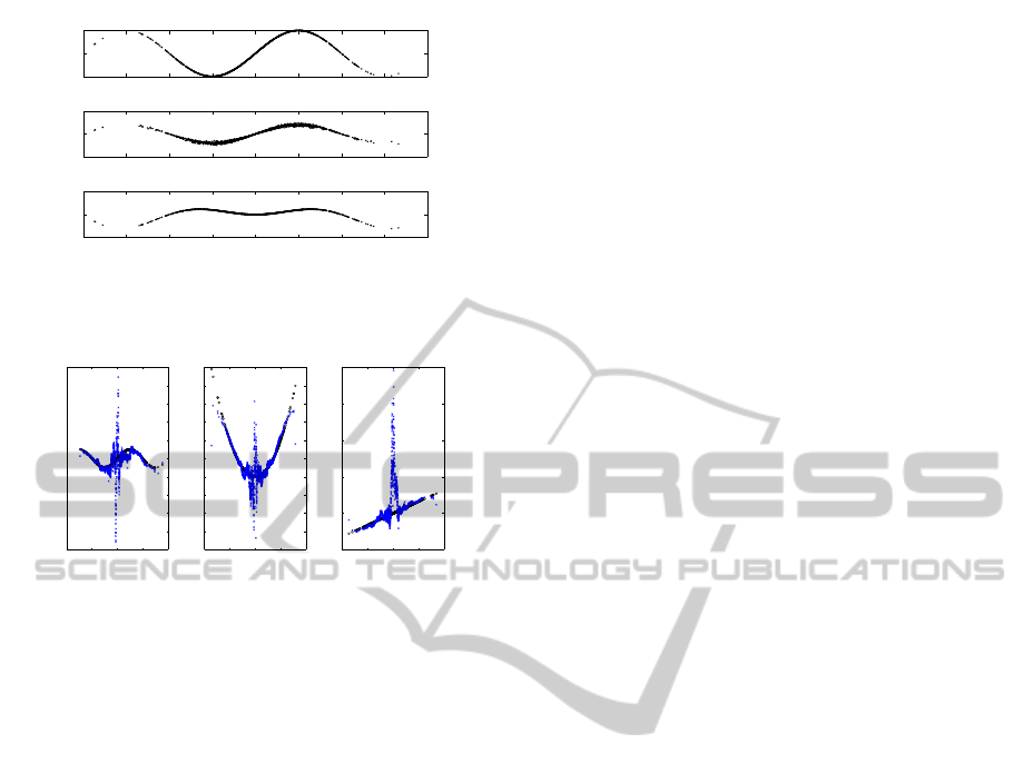
Now, the detailed process from equations (5) to (8)

is implemented and, in order to understand how the

0 500 1000 1500

−20

Ordered data

mdv

0 500 1000 1500

−5

0 500 1000 1500

−20

Reordered data

0 500 1000 1500

−5

Figure 3: Temporally ordered data (left) an the effect of the

reordering process for y

mdv

reordering process is useful to detect state-parameter

dependence, the ﬁrst iteration of the ﬁrst parameter is

detailed. The modiﬁed dependent variable y

mdv

, cor-

responding to the ﬁrst parameter ρ

is:

mdv

(k) = y(k)−ρ

(k)} u

(k− 1)−ρ

(k)} u

(k− 1)

(16)

The signal y

mdv

is the measure y without the ef-

fect provided by the parameters ρ

and ρ

, each one

multiplied by the regressors z

and z

, respectively.

The modiﬁed dependent variable in the reordered

space corresponding to the ﬁrst transformed param-

eter y

mdv

→ y

∗

mdv

is:

∗

mdv

(k) = ρ

∗

(k){x

∗

(k)} u

∗

(k− 1) (17)

We can say that the relationship y

∗

mdv

has only the

ﬁrst parameter effect. Then the relation among x

∗

and

∗

mdv

shows the shape of the dependence between x

and ρ

after of the reordering process. This effect is

shown in Fig. 3: The original sinusoidal shape of the

state-parameter dependence ρ

is evident after de re-

ordering of y

mdv

based on the ascendant value of the

state x

This process should be repeated for the other pa-

rameters ρ

and ρ

iteratively. Only for the ﬁrst iter-

ation ρ

first

, i = 1, 2, 3, is used. A stopping criteria for

the algorithm should be a maximum iteration num-

ber or a minimal difference in two sequential estima-

tions of ρ

; in our tests 40 iterations were used for

each case to contrast our results. This example was

implemented in the INCA toolbox, for the cases of

ﬁlter factor α = 0.9 and α = 0.95. The state-parameter

dependence non-parametrically estimated is shown in

Fig. 4.

In order to contrast graphically our dependence

estimation, Fig. 5 shows the state-parameter depen-

dences estimation using the function

sdp.m

of CAP-

TAIN. Note the differences of ﬁgures 4 and 5 espe-

cially on the low data density regions. The Table 1

shows results of the state-parameter dependency for

the three unknown parameters using the INCA tool-

box, i.e with low and ﬁxed α, and the CAPTAIN tool-

box, i.e. with optimized α.

Off-lineState-dependentParameterModelsIdentificationusingSimpleFixedIntervalSmoothing

339

−4 −2 0 2 4

0.5

1.5

2.5

3.5

−5 0 5

−2

−5 0 5

Figure 4: SDP estimation using the INCA for α = 0.95

(blue) and reference (black).

−5 0 5

1.5

2.5

3.5

−5 0 5

Figure 5: SDP estimation using the CAPTAIN (blue) and

the reference (black).

Table 1: Estimation error of the state-parameter dependency

using the INCA and CAPTAIN toolboxes.

SDP Method α MAE(

− ρ

) Time[s]

INCA 0.90 0.4423 16

INCA 0.95 0.2917 15

CAPTAIN - 0.7564 31

INCA 0.90 0.4267 16

INCA 0.95 0.3104 15

CAPTAIN - 0.2956 31

INCA 0.90 0.2521 16

INCA 0.95 0.1665 15

CAPTAIN - 0.2847 31

4.1 Estimation of ARX-SDP Model with

Unitary Regressors

Now we consider the ARX-SDP model with unitary

regressors:

y(k) = ρ

(k)} + ρ

(k)}

+ρ

(k)} + e(k) (18)

The dependences to be estimate are:

(k)} = u

(k− 1)



sin



(k− 1)



+ 2



(k)} = u

(k− 1)



(k− 1)+ 1



(k)} = u

(k− 1)(0.8x

(k− 1)+ 3)

The modiﬁed dependent variable y

mdv

in this case is

simply:

−5 0 5

−4

−2

−5 0 5

−14

−12

−10

−8

−6

−4

−2

−5 0 5

Figure 6: SDP estimation using the INCA toolbox, when

model has unitary regressors (blue) and reference (black).

mdv

(k) = y(k) −

(k) +

(k) (19)

Notice that y

mdv

is exactly the measurement signal

without the other two parameters effect

and

Then the signal y

mdv

should have shape similarity

with the ﬁrst parameter ρ

. In the previous case, we

can say that y

mdv

also have ρ

information but per-

turbed by the regressor effects z

, see equations (16)

and (17). The dependence estimation result of this

case is shown in Fig. 6.

We recommend to select a model with unitary re-

gressors when the state-regressor dependence shape is

more important than its exact value. e.g. in the case of

parametric fault detection it could be more important

to monitor the structure invariance of the model than

its exact parameter value.

4.2 Estimation of ARX-SDP Model with

Equal Regressors and States

Finally we consider ARX-SDP model with correlated

regressors and states, exactly z

= x

y(k) = ρ

(k)} x

(k− 1)+ ρ

(k)} x

(k− 1)

+ρ

(k)} x

(k− 1)+ e(k) (20)

Notice that in equations (12) both signals are uncorre-

lated then the product of them keep, in some manner,

the shape of the unknownparameter. In (20) the shape

is completely affected because the parameter and the

regressor are correlated. Thus, ρ

(k)} x

(k−1) has a

completely different shape from parameter ρ

(k)}.

In the models 12 and 18 the parameters and states

were uncorrelated and their product shapes was con-

served. For this case the modiﬁed dependent variable

for the ﬁrst parameter ρ

is:

mdv

(k) = ρ

(k)} x

(k) (21)

= x

(k)sin



(k)



+ 2x

(k) (22)

and its sinusoidal form isn’t maintained, because

the regressor x

(k) is correlated with the parameter

ICINCO2015-12thInternationalConferenceonInformaticsinControl,AutomationandRobotics

340

−4 −3 −2 −1 0 1 2 3 4

−1

original dependence

−4 −3 −2 −1 0 1 2 3 4

−5

uncorrelated product

−4 −3 −2 −1 0 1 2 3 4

−5

correlated product

Figure 7: Original state-parameter dependence (top) and re-

lation between state and regressor-parameter product, when

the factors are uncorrelated (middle) and correlated (below).

−4 −2 0 2 4

−10

−8

−6

−4

−2

−4 −2 0 2 4

−8

−6

−4

−2

−4 −2 0 2 4

−5

Figure 8: SDP estimation using the INCA toolbox, when

state and parameter are correlated.

(k)}, see Fig. 7. Finally Fig. 8 shows the SDP

estimation for the three parameters when regressors

and parameters are correlated.

5 CONCLUSIONS

Inspired on Young’s algorithm, temporal data re-

ordering strategy to reduce the data entropy, the

state-parameter dependence estimation for ARX-SDP

model is studied in this paper. Firstly, we proposed a

ﬁxed and relatively low value of the forgetting factor

α instead of considering its optimal value. It showed

a good estimation performance especially in the low

density regions. It is because after de reordering pro-

cess, the low density data is averaged with the high

state density.

In spite of our proposal do not result in smoother

state-parameter dependency as in CAPTAIN, this is

not disadvantageous, because it is still necessary a pa-

rameterization stage, e.g. by using support vector re-

gression (Alegria, 2015a). An important consequence

of our proposal, low and ﬁxed forgetting factor, is the

ﬂexibility to structural changes that our parameter-

state dependency algorithm presents. This is very im-

portant for a future On-Line version of SDP estima-

tion.

The three ARX-SDP estimation examples showed

the usefulness of our proposal and implementation for

the SFIS algorithm. For the ﬁrst case the parame-

ter and regressor are uncorrelated, and the SDP es-

timation results were good. For the second case with

unitary regressors the SDP estimation results are also

very good but with offsets. For the third case when

the parameters and regressors are correlated the SDP

estimation is poor. It is interesting to observe that, for

the three parameters, the SDP estimation around the

zero state has greater errors. This is due to the very

low value of the regressor-parameter product that re-

duces the data richness.

ACKNOWLEDGEMENTS

We thank Brazilian agency CAPES for the ﬁnancial

support.

REFERENCES

Alegria, E. J. (2015a). State-dependent parameter models

identiﬁcation using data transformations and support

vector regression. In 12th International Conference

on Informatics in Control, Automation and Robotics

ICINCO.

Alegria, E. J. (2015b). State dependent parameters on-line

estimation for nonlinear regression models. Master’s

thesis, Universidade estadual de Campinas - UNI-

CAMP.

F. Previdi, M. L. (2003). Identiﬁcation of a class of non-

linear parametrically varying models. International

Journal of Adaptive Control and Signal Processing,

17:33–50.

Hu, J., Kumamura, K., and Hirasawa, K. (2001). A quasi-

ARMAX approach to modeling of nonlinear systems.

International Journal of Control, 74:1754–1766.

Jazwinski, A. H. (2007). Stochastic Processes and Filtering

Theory. Dover publications.

Priestley, M. (1988). Non-linear and non-stationary time

series analysis. Academic Press, London.

Taylor, C., Pedregal, D., Young, P., and Tych, W. (2007).

Environmental time series analysis and forecasting

with the captain toolbox. Environmental Modelling

& Software, 22(6):797–814.

Yaakov Bar-Shalom, X. Rong Li, T. K. (2001). Estimation

with Applications to Tracking and Navigation. John

Wiley& Sons, Inc. cop., New York (N.Y.), Chichester,

Weinheim.

Young, P., McKenna, P., and Bruun, J. (2001). Identiﬁca-

tion of non-linear stochastic systems by state depen-

dent parameter estimation. International Journal of

Control, 74(18):1837–1857.

Young, P. C. (2011). Recursive Estimation and Time-Series

Analysis. Springer-Verlag, 2 edition.

Off-lineState-dependentParameterModelsIdentificationusingSimpleFixedIntervalSmoothing

341