Elliptical and Archimedean Copulas

in Estimation of Distribution Algorithm with Model Migration

Martin Hyr

s and Josef Schwarz

Faculty of Information Technology, Brno University of Technology, Bo

zet

echova 2, Brno, Czech Republic

Keywords:

Estimation of Distribution Algorithms, Copula Theory, Parallel EDA, Island-based Model, Multivariate

Copula Sampling, Migration of Probabilistic Models.

Abstract:

Estimation of distribution algorithms (EDAs) are stochastic optimization techniques that are based on building

and sampling a probability model. Copula theory provides methods that simplify the estimation of a probabil-

ity model. An island-based version of copula-based EDA with probabilistic model migration (mCEDA) was

tested on a set of well-known standard optimization benchmarks in the continuous domain. We investigated

two families of copulas – Archimedean and elliptical. Experimental results conﬁrm that this concept of model

migration (mCEDA) yields better convergence as compared with the sequential version (sCEDA) and other

recently published copula-based EDAs.

1 INTRODUCTION

Estimation of distribution algorithms (EDAs) belong

to a new class of evolutionary optimization meth-

ods that explore the search space by estimating and

sampling an explicit probabilistic model of promis-

ing solutions. EDAs applied to discrete problems

are described in the well-known papers UMDA (Pe-

likan and M

uhlenbein, 1999b), BMDA (Pelikan and

uhlenbein, 1999a), MIMIC (De Bonet et al., 1997),

and BOA (Pelikan et al., 1999). Solutions of the op-

timization problems in the real value domain can be

found in (Larra

naga and Lozano, 2001). A very mod-

ern and accessible survey of the EDAs algorithm is

presented in (Hauschild and Pelikan, 2011).

The main advantage of EDAs is its capacity to dis-

cover those variable linkages that yield a solution to a

complex optimization problem. On the one hand this

probability model-based approach has allowed EDAs

to be applied to large and complex problems. On

the other hand explicit probabilistic models are very

time consuming. That was the reason for implement-

ing various advanced EDAs to solve this problem.

The well-known enhancement approaches include the

parallelization of model building and sporadic model

building (Hauschild and Pelikan, 2011).

In the last ten years a new approach has appeared

to building an efﬁcient probabilistic model that is

based on copula theory (Mai and Scherer, 2012).

Copulas are special probability distribution functions.

Due to their properties it is possible to use them

to model correlations within multivariate problems –

the joint distribution is separated into the univariate

marginal distributions and into the correlation struc-

ture that is expressed by the copula function. Cop-

ula theory has very often been used in ﬁnance and

statistics works (Nelsen, 2006; Cherubini et al., 2004;

Aas et al., 2009) (e.g. modeling health insurance data

(Zimmer and Trivedi, 2006)).

Recently copulas have been utilized in the ﬁeld of

the machine learning (Rey and Roth, 2012; P

oczos

et al., 2012). More recently the copula theory has

been applied to EDA probability models. The sim-

plest case is the application with bivariate (2D) copu-

las: (Wang et al., 2009) – 2D Gaussian copula EDA,

(Wang et al., 2010b) – 2D Clayton copula EDA,

(Wang et al., 2010a) – 2D Gumbel copula EDA.

In the case of multivariate models bivariate cop-

ulas are used as local building blocks in vari-

ous graph dependence structures: (Salinas-Guti

errez

et al., 2009) – MIMIC + Frank and Gaussian copula),

endez and Landa, 2012) – Bayesian network +

Archimedean copulas, (Salinas-Guti

errez et al., 2011)

– D-vine + copulas, (Soto et al., 2012) – C-vine, D-

vine + copulas.

The copula-based EDA starts with an estimation

of the marginal distribution of each variable, then us-

ing a proper copula, the joint distribution is estab-

lished. Given the margins and a copula, it is then pos-

sible to generate new solutions.

212

Hyrš, M. and Schwarz, J..

Elliptical and Archimedean Copulas in Estimation of Distribution Algorithm with Model Migration.

In Proceedings of the 7th International Joint Conference on Computational Intelligence (IJCCI 2015) - Volume 1: ECTA, pages 212-219

ISBN: 978-989-758-157-1

This paper deals with an efﬁcient parallelization

of island-based mCEDA with the goal to increase

the convergence speed. After some experiments we

chose the island-based structure with bidirectional

ring topology. Instead of the often used migration of

individuals we instantiated the migration of probabil-

ity models. Note that the ﬁrst experiments with this

new concept were published in (delaOssa et al., 2004;

Schwarz and Jaro

s, 2008) for the optimization in the

discrete domain, the chief obstacle being an efﬁcient

combination of the probabilistic models, especially

those having the dependence structure expressed by

a graph. That is why we focused on the migration of

probabilistic model parameters only.

The paper is organized as follows. In Section 2,

the basis of copula theory is given. In Section 3, the

utilization of copulas in EDA is described, and sam-

pling algorithms for copulas are presented. In Sec-

tion 4, the island-based model of evolution algorithm

with copula-model migration is described. Our exper-

iments are discussed in Section 5. The conclusions

are given in Section 6.

2 COPULA THEORY

The copula concept was introduced by (Sklar, 1959)

in order to separate the effect of dependence of vari-

ables from the effect of marginal distributions in a

joint distribution. A copula is a function which joins

the univariate distribution function and creates mul-

tivariate distribution functions. This approach allows

us to transform multivariate statistic problems into the

univariate problems with the relation represented by

just the copula.

Deﬁnition. A copula C is a multivariate probability

distribution function for which the marginal probabil-

ity distribution of each variable is uniform in [0; 1].

Deﬁnition. A copula is a function C : [0; 1]

→ [0; 1]

with the following properties:

1. C(u

, u

, . . . , u

) = 0 for at least one u

= 0

2. C(1, 1, . . . , 1, u

, 1, . . . , 1) = u

for all i = 1, 2, . . . , d

3. C(u

, u

, . . . , u

) is d-increasing (see lit. for de-

tails)

Theorem. Sklar’s theorem: Let F be a d-dimensional

distribution function with margins F

, . . . , F

. Then

there exists a d-dimensional copula C such that for

all (x

, . . . , x

) ∈ R

it holds that

F(x

, . . . , x

) = C (F

), . . . , F

)) (1)

If F

, . . . , F

are continuous, then C is unique. Con-

versely, if C is a d-dimensional copula and F

, . . . , F

0.1

0.2

0.3

0.4

0.5

0.6

0.7

0.8

0.9

0 0.1 0.2 0.3 0.4 0.5 0.6 0.7 0.8 0.9 1

0.1

0.2

0.3

0.4

0.5

0.6

0.7

0.8

0.9

0 0.1 0.2 0.3 0.4 0.5 0.6 0.7 0.8 0.9 1

0.1

0.2

0.3

0.4

0.5

0.6

0.7

0.8

0.9

0 0.1 0.2 0.3 0.4 0.5 0.6 0.7 0.8 0.9 1

0.1

0.2

0.3

0.4

0.5

0.6

0.7

0.8

0.9

0 0.1 0.2 0.3 0.4 0.5 0.6 0.7 0.8 0.9 1

0.1

0.2

0.3

0.4

0.5

0.6

0.7

0.8

0.9

0 0.1 0.2 0.3 0.4 0.5 0.6 0.7 0.8 0.9 1

0.1

0.2

0.3

0.4

0.5

0.6

0.7

0.8

0.9

0 0.1 0.2 0.3 0.4 0.5 0.6 0.7 0.8 0.9 1

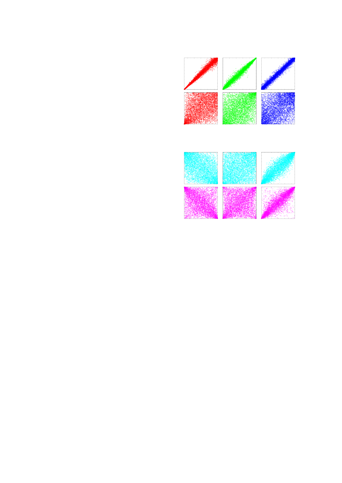
Figure 1: Scatterplots of bivariate Archimedean copulas:

Clayton (left), Gumbel (middle) and Frank (right) with de-

pendence strengths 0.9 (top) and 0.3 (bottom).

0.1

0.2

0.3

0.4

0.5

0.6

0.7

0.8

0.9

0 0.1 0.2 0.3 0.4 0.5 0.6 0.7 0.8 0.9 1

0.1

0.2

0.3

0.4

0.5

0.6

0.7

0.8

0.9

0 0.1 0.2 0.3 0.4 0.5 0.6 0.7 0.8 0.9 1

0.1

0.2

0.3

0.4

0.5

0.6

0.7

0.8

0.9

0 0.1 0.2 0.3 0.4 0.5 0.6 0.7 0.8 0.9 1

0.1

0.2

0.3

0.4

0.5

0.6

0.7

0.8

0.9

0 0.1 0.2 0.3 0.4 0.5 0.6 0.7 0.8 0.9 1

0.1

0.2

0.3

0.4

0.5

0.6

0.7

0.8

0.9

0 0.1 0.2 0.3 0.4 0.5 0.6 0.7 0.8 0.9 1

0.1

0.2

0.3

0.4

0.5

0.6

0.7

0.8

0.9

0 0.1 0.2 0.3 0.4 0.5 0.6 0.7 0.8 0.9 1

Figure 2: Scatterplots of bivariate eliptical copulas: Gaus-

sian (top) and Student, ν = 2 (bottom), with dependence

strengths −0.5 (left), 0.3 (middle) and 0.9 (right).

are univariate distribution functions, then the func-

tion F deﬁned via (1) is a d-dimensional distribution

function.

In this paper we focus on two big copula families

– Archimedean and elliptic.

Archimedean copulas are capable of capturing

wide ranges of dependence. The deﬁnition of the

Archimedean copula is based on the generator func-

tion. There are many existing Archimedean copulas

and many more that could be created. The three cop-

ulas, i.e. Clayton, Gumbel and Frank appear regu-

larly in statistics literature, they are popular because

they model different patterns of dependence and have

a relatively simple functional form. Fig. 1 shows scat-

terplots of these copulas.

The elliptical copulas are derived from the related

elliptical distribution. The ﬁrst example of elliptical

copula is the Gaussian copula, which belongs to the

normal distribution, the second example is the Stu-

dent copula, which belongs to the t-distribution (see

Fig. 2).

Elliptical and Archimedean Copulas in Estimation of Distribution Algorithm with Model Migration

213

3 COPULA-BASED ESTIMATION

OF DISTRIBUTION

ALGORITHM

Estimation of distribution algorithms belongs to the

advanced evolutionary algorithms. Solving the nu-

merical optimization problem, vector x = (x

, . . . , x

)

of the optimal solution is searched out.

The core of the canonical EDA consists of three

main steps, see Algorithm 1.

Algorithm 1: The pseudocode of canonical EDA.

Generate initial population.

WHILE (termination criteria is false):

1. Select promising solutions into subpopulation

from the current population.

2. Create the probability model from the selected

subpopulation.

3. Sample the probability model and generate the

new population.

Step 1 is quite straightforward, the promising so-

lutions are stated using the standard selection trunca-

tion. In the case of copula-based EDA it is neces-

sary to choose the proper type of copula and derive

the copula parameters and the marginal distribution

parameters.

The principle of sampling schema for generating

the new individuals using the copula model is de-

scribed in Algorithm 2:

Algorithm 2: Sampling the copula and generating the new

individuals.

1. Obtain the random copula sample (u

, . . . , u

) ∼

C, where u

∈ [0; 1].

2. Derive the vector x of the searched solution using

inverse marginal distributions, x

= F

−1

3.1 Identiﬁcation of Copula Probability

Model

The copula-based probability model includes two

parts: univariate marginal distributions and the cop-

ula function. Marginal distributions can be identiﬁed

separately for each variable and the copula includes

the correlation between variables.

For marginal distribution in each dimension i =

1, . . . , d we used normal distribution, which is param-

eterized by the mean value µ

and standard deviation

For assessing the parameters of the copula we

used the Kendall τ correlation coefﬁcient.

In the case of Archimedean copulas the following

relations hold for the parameter θ (in the case of d-

variate copulas, d ≥ 3, we use average

τ; for d = 2

the standard pairwise τ is used):

• for the Clayton copula θ

Clayton

2τ

1−τ

• for the Gumbel copula θ

Gumbel

1−τ

• for the Frank copula (approximation) θ

Frank

(10

arcsin(τ)

− 1) e.

Elliptical copulas are parameterized by correlation

matrix R. Elements R

i j

are adapted from Kendall’s τ

for each pair of dimensions i, j using formula R

i j

sin

πτ

i j

3.2 Copula Sampling Algorithms

Now we specify step 1 from Alg. 2 for each type of

copulas in more details.

The algorithm for sampling Archimedean copu-

las uses a random value J, which is obtained from the

distribution given by the inverse of Laplace transform

−1

of generator (Mai and Scherer, 2012; Aas, 2004;

Melchiori, 2006), see Alg. 3.

Algorithm 3: Archimedean copula sampling.

1. generate value J ∼ L

−1

[ϕ(t)]

2. generate uniformly distributed random numbers

∼ U (0, 1) (for i = 1, . . . , d)

3. return u

= ϕ



−log(z

)



(for i = 1, . . . , d)

According to (Aas, 2004; Melchiori, 2006) the

value of J can be derived:

• for the Clayton copula by Gamma distribution J ∼

Gamma



, θ



• for the Gumbel copula by Levy skew alpha-Stable

distribution J ∼ Stable



, 1,



cos

2θ



, 0



• for the Frank copula by logarithmic series distri-

bution J ∼ Logarithmic



1 − e

−θ



The sampling scheme for Gaussian and Student

copulas (Mai and Scherer, 2012) (see Alg. 4, 5) uses

the Cholesky decomposition of the given correlation

matrix R to obtain the lower triangular matrix L, such

that LL

= R. The Student copula is further speciﬁed

by degrees of freedom, we use ν = (N − 1)d (where

N is population size and d number of dimensions).

ECTA 2015 - 7th International Conference on Evolutionary Computation Theory and Applications

214

Algorithm 4: Gaussian copula sampling.

1. compute L

2. generate random numbers z

∼ No(0, 1) with stan-

dard normal distribution (for i = 1, . . . , d)

3. calculate s

∑

j=1

i, j

(for i = 1, . . . , d)

4. return u

= Φ(s

) (for i = 1, . . . , d)

Algorithm 5: Student copula sampling.

1. compute L

2. generate V ∼ χ

(ν)

3. generate random numbers z

∼ No(0, 1) with stan-

dard normal distribution (for i = 1, . . . , d)

4. calculate s

∑

j=1

i, j

(for i = 1, . . . , d)

5. return u

= t

) (for i = 1, . . . , d)

4 ISLAND-BASED COPULA-EDA

The principal motivation for the proposal of a concept

of copula-based EDA parallelization is to discover the

efﬁciency of the transfer of probabilistic parameters

instead of the traditional transfer of individuals. The

main goal is to improve algorithm convergence. In the

case of EDAs only a few papers deal with the discrete

probability model migration (delaOssa et al., 2004;

delaOssa et al., 2005) and (Hyr

s and Schwarz, 2014)

in the case of copula-based EDA.

4.1 EDA with Migration

With the concordance of experimental work done in

(Schwarz and Jaro

s, 2008), and according to our ex-

perimental results, we used the island-based commu-

nication model with bidirectional ring topology. This

topology provides good local interaction and in a few

steps allows the propagation of information along the

ring.

The evolution process on every island runs inde-

pendently. When the migration condition is met the

communication (transfer of model parameters) is ac-

tivated, see Alg. 6.

4.2 Model Combination

According to the island-based topology we have de-

composed the migration process into pairwise inter-

actions of two islands – one of them is the resident

island speciﬁed by resident probabilistic model M

Algorithm 6 : The pseudocode of canonical EDA with

model migration.

1. Generate initial populations.

2. FOR each island DO IN PARALLEL:

3. WHILE (termination criteria is false):

4. Select promising individuals

5. Create probability model (see Sec. 3)

6. IF (sending condition):

7. Send model

8. WHILE (immigrant model received):

9. Combine models (see Sec. 4.2)

10. Sample new population from probability model

and the other one is the immigrant island whose prob-

abilistic model M

is transferred to a new resident

model.

The combination of the immigrant model with the

model of the resident island is described in more de-

tails. In general, the modiﬁcation of the resident

model by the immigrant model can be formalized by

(Schwarz and Jaro

s, 2008):

new

= (1 − β)M

+ βM

(2)

where the coefﬁcient β ∈ [0;1] speciﬁes the inﬂuence

of the immigrant model.

We have proposed the following model combina-

tion rules according to (Fr

uhwirth-Schnatter, 2006):

• Learning the mean value µ

of each univariate

marginal distribution F

)

new

= (1 − β)µ

+ βµ

(3)

• Learning the standard deviation σ

of each uni-

variate marginal distribution F

)

new

(1 − β)





new

− µ









+β





new

− µ









(4)

• Learning the correlation matrix value R

i j

new

i j

= (1 − β)R

i j

+ βR

i j

(5)

We have chosen the coefﬁcient β as

β =

(

f it

+ f it

f it

≤ f it

0.1 otherwise

(6)

where f it

or f it

represents the ﬁtness value of the

resident or the immigrant model.

Elliptical and Archimedean Copulas in Estimation of Distribution Algorithm with Model Migration

215

5 EXPERIMENT AND RESULTS

We used standard benchmark problems to compare

island-based copula-EDA (mCEDA) with the sequen-

tial one (sCEDA).

5.1 Benchmarks

The shifted variants of several well-known bench-

marks from the area of numerical optimization are

used. All these functions have been adapted such that

the task is minimization with optimal ﬁtness value 0

and with shifted optima position.

• Elliptic Function:

f (x) =

∑

i=1

(10

)

i−1

d−1

, x

∈ [−100; 100]

• Rastrigin’s Function:

f (x) =

∑

i=1



− 10 cos(2πx

) + 10



, x

∈ [−5;5]

• Ackley’s Function:

f (x) = −20 e

−0.2

∑

i=1

− e

∑

i=1

cos(2πx

)

20 + e, x

∈ [−32; 32]

• Schwefel’s Problem 1.2:

f (x) =

∑

i=1



∑

j=1



, x

∈ [−100; 100]

• Rosenbrock’s Function:

f (x) =

∑

d−1

i=1



100(x

− x

i+1

)

+ (x

− 1)



∈ [−100; 100]

• Summation Cancellation:

f (x) = 10

−

−5

∑

i=1

∑

j=1

, x

∈ [−1; 1]

We used the shifted optima position in the form

f itness(x) = f (x

), where x

= x

− 0.25(x

max

−

min

), i = 1, . . . , d.

We have chosen the following settings:

• Problem size: 10 variables/dimensions for all

problems.

• Population size of each island: 500.

• Selection: We used truncation selection, with a

selection proportion of 0.2, i.e. 100 individuals.

• Number of islands: 10.

• Migration rate: after every 20 generations.

• Maximum number of ﬁtness evaluations: 500000

(i.e. 100 generations for the island-based model

and 1000 generations for the sequential variant).

• Number of independent runs: 20.

5.2 Results and Discussion

We carried out a comparison of two variants of

the copula-based EDA algorithm: sequential variant

sCEDA speciﬁed in Sec. 3 and island-based algorithm

with model migration mCEDA (Sec. 4) – both of them

with the same classes of copulas.

We used the so-called weak model of paralleliza-

tion, the population size in sCEDA is equal to the pop-

ulation of one island in mCEDA. The total population

in mCEDA is thus ten-times bigger than in sCEDA.

To retain the same computational cost, we increased

the number of generations ten-times for sCEDA ac-

cording to mCEDA, thus the total computational cost

measured by ﬁtness evaluations is the same.

In Tables 1–6 the convergence of the proposed

sCEDA and mCEDA algorithms is presented. The

mean values related to speciﬁed evaluation epochs are

listed.

It can be seen that mCEDA performs better than

sCEDA for most benchmarks. (Only in the case of

Ackley’s benchmark the sCEDA is better, the cause is

under our investigation.) The sCEDA is able to ﬁnd

a relatively good local solution quite fast but then it

loses its diversity and no further improvement is ob-

tained. The mCEDA converges slowly but it has the

capability to ﬁnd near optimal solution. We suppose

that this performance is caused by the phenomenon of

the proposed model migration.

In the case of Rosenbrock’s and Summation Can-

cellation problems, only mCEDA using elliptic copu-

las is able to achieve some progress during the evo-

lution process. Neither Archimedean copulas nor

sCEDA have this capacity.

Besides the comparison of sCEDA and mCEDA

the inﬂuence of each copula type in mCEDA is worth

discussing. In the case of Rosenbrock’s and Sum-

mation Cancellation, only elliptical copulas are able

to perform well. In the case of Rastrigin’s and El-

liptic functions, Archimedean copulas perform better

than elliptic ones. In the case of Ackley’s and Schwe-

fel’s 1.2 functions, there is no signiﬁcant difference

between the two copula families.

From the observations it follows that the success

rate of the both versions of mCEDA is almost iden-

tical. But in the case of Archimedean mCEDA the

drawback appears in tendency to become stuck on lo-

cal optima, see Table 3.

In Tables 7–9 we arranged a comparison (mean

ﬁtness values) of mCEDA using the Frank copula

(mCEDA-F) and the Gaussian copula (mCEDA-G)

(as members of Archimedean and elliptic families)

with the other published algorithms that used differ-

ent versions of copulas. The comparison is done for

the same number of ﬁtness evaluations for the same

subset of benchmarks with 10 dimensions.

In Table 7 a comparison with the algorithm using

the Copula Bayesian network (M

endez and Landa,

ECTA 2015 - 7th International Conference on Evolutionary Computation Theory and Applications

216

Table 1: Experimental results (mean ﬁtness) for Rastrigin’s

function.

ﬁt. eval. Clayton Gumbel Frank Gauss Student

island based

100000 5.78e+00 1.42e-01 9.88e-02 2.47e+01 2.49e+01

200000 3.70e-05 1.04e-07 3.92e-07 1.16e+00 1.70e+00

300000 2.79e-11 2.72e-14 2.23e-13 2.41e-01 4.26e-01

400000 0.00e+00 0.00e+00 0.00e+00 5.02e-02 9.60e-02

500000 0.00e+00 0.00e+00 0.00e+00 1.71e-04 5.00e-02

sequential

100000 2.56e-01 4.65e-01 8.67e-01 2.36e+00 2.75e+00

200000 2.56e-01 4.65e-01 6.52e-01 2.36e+00 2.75e+00

300000 2.56e-01 4.65e-01 6.52e-01 2.36e+00 2.75e+00

400000 2.56e-01 4.65e-01 6.52e-01 2.36e+00 2.75e+00

500000 2.56e-01 4.65e-01 6.52e-01 2.36e+00 2.75e+00

Table 2: Experimental results (mean ﬁtness) for Rosen-

brock’s function.

ﬁt. eval. Clayton Gumbel Frank Gauss Student

island based

100000 8.40e+00 8.40e+00 8.57e+00 8.13e+00 8.27e+00

200000 7.83e+00 7.89e+00 8.00e+00 6.79e+00 6.59e+00

300000 7.66e+00 7.76e+00 7.86e+00 6.46e+00 6.16e+00

400000 7.53e+00 7.62e+00 7.69e+00 6.25e+00 5.86e+00

500000 7.50e+00 7.60e+00 7.66e+00 6.20e+00 5.82e+00

sequential

100000 8.27e+00 8.13e+00 8.14e+00 3.28e+04 7.63e+04

200000 8.27e+00 8.13e+00 8.14e+00 3.28e+04 7.61e+04

300000 8.27e+00 8.13e+00 8.14e+00 3.28e+04 7.61e+04

400000 8.27e+00 8.13e+00 8.14e+00 3.28e+04 7.61e+04

500000 8.27e+00 8.13e+00 8.14e+00 3.28e+04 7.61e+04

Table 3: Experimental results (mean ﬁtness) for Summation

Cancellation function.

ﬁt. eval. Clayton Gumbel Frank Gauss Student

island based

100000 1.00e+05 1.00e+05 1.00e+05 9.99e+04 9.98e+04

200000 9.99e+04 9.99e+04 9.99e+04 9.43e+04 9.64e+04

300000 9.99e+04 9.97e+04 9.97e+04 7.66e+04 6.89e+04

400000 9.97e+04 9.95e+04 9.92e+04 5.23e+04 4.53e+04

500000 9.97e+04 9.93e+04 9.90e+04 4.46e+04 4.40e+04

sequential

100000 1.00e+05 1.00e+05 1.00e+05 9.99e+04 1.00e+05

200000 1.00e+05 1.00e+05 1.00e+05 9.99e+04 1.00e+05

300000 1.00e+05 1.00e+05 1.00e+05 9.99e+04 1.00e+05

400000 1.00e+05 1.00e+05 1.00e+05 9.99e+04 1.00e+05

500000 1.00e+05 1.00e+05 1.00e+05 9.99e+04 1.00e+05

2012) after 100,000 evaluations is shown. For the

case of Rastrigin’s, Ackley’s and Schwefel’s 1.2 func-

tions mCEDA-F and mCEDA-G are evidently better,

for Rosenbrock’s function the results are comparable.

Table 4: Experimental results (mean ﬁtness) for Elliptic

function.

ﬁt. eval. Clayton Gumbel Frank Gauss Student

island based

100000 2.76e-01 3.35e-01 3.42e-01 2.78e+01 4.25e+01

200000 4.94e-08 5.78e-08 8.14e-08 5.28e+00 4.67e-01

300000 6.75e-15 1.02e-14 1.46e-14 1.94e+00 1.82e-01

400000 3.82e-17 4.27e-17 1.21e-18 1.39e+00 1.32e-01

500000 3.82e-17 4.27e-17 1.21e-18 9.63e-01 1.17e-01

sequential

100000 6.46e-16 7.23e-16 6.68e-16 1.30e+03 2.45e+03

200000 6.46e-16 7.23e-16 6.68e-16 1.30e+03 2.45e+03

300000 6.46e-16 7.23e-16 6.68e-16 1.30e+03 2.45e+03

400000 6.46e-16 7.23e-16 6.68e-16 1.30e+03 2.45e+03

500000 6.46e-16 7.23e-16 6.68e-16 1.30e+03 2.45e+03

Table 5: Experimental results (mean ﬁtness) for Ackley’s

function.

ﬁt. eval. Clayton Gumbel Frank Gauss Student

island based

100000 1.16e-02 1.17e-02 1.35e-02 1.27e-02 1.33e-02

200000 4.91e-06 4.39e-06 5.85e-06 5.65e-06 5.53e-06

300000 2.01e-09 2.16e-09 2.51e-09 2.36e-09 2.00e-09

400000 8.67e-13 8.40e-13 1.15e-12 8.48e-13 7.40e-13

500000 1.33e-15 1.69e-15 2.93e-15 9.77e-16 1.51e-15

sequential

100000 0.00e+00 0.00e+00 0.00e+00 3.21e-02 8.60e-02

200000 0.00e+00 0.00e+00 0.00e+00 3.21e-02 8.60e-02

300000 0.00e+00 0.00e+00 0.00e+00 3.21e-02 8.60e-02

400000 0.00e+00 0.00e+00 0.00e+00 3.21e-02 8.60e-02

500000 0.00e+00 0.00e+00 0.00e+00 3.21e-02 8.60e-02

Table 6: Experimental results (mean ﬁtness) for Schwefel’s

1.2 function.

ﬁt. eval. Clayton Gumbel Frank Gauss Student

island based

100000 1.78e-03 1.79e-03 2.20e-03 2.85e-03 2.54e-03

200000 1.03e-10 9.30e-11 1.11e-10 2.63e-10 2.48e-10

300000 5.09e-17 7.49e-17 1.08e-16 2.07e-16 2.85e-16

400000 5.09e-17 7.49e-17 1.08e-16 2.07e-16 2.85e-16

500000 5.09e-17 7.49e-17 1.08e-16 2.07e-16 2.85e-16

sequential

100000 6.15e-16 5.39e-16 6.00e-16 5.47e+01 2.23e+02

200000 6.15e-16 5.39e-16 6.00e-16 5.46e+01 2.23e+02

300000 6.15e-16 5.39e-16 6.00e-16 5.46e+01 2.23e+02

400000 6.15e-16 5.39e-16 6.00e-16 5.46e+01 2.23e+02

500000 6.15e-16 5.39e-16 6.00e-16 5.46e+01 2.23e+02

In Table 8 a comparison with the other suite of

algorithms (Zhao and Wang, 2012; Jia et al., 2013)

is carried out on the level of 300,000 evaluations.

In the case of Rosenbrock’s function the results are

Elliptical and Archimedean Copulas in Estimation of Distribution Algorithm with Model Migration

217

Table 7: Comparison (mean ﬁtness) of mCEDA with Cop-

ula Bayesian Network (CBN) from (M

endez and Landa,

2012).

Rastr. Ack. Schw. 1.2 Rosen.

CBN 2.39e+00 3.71e-02 2.23e+01 1.05e+01

mCEDA-F 9.88e-02 1.35e-02 2.20e-03 8.57e+00

mCEDA-G 2.47e+01 1.27e-02 2.85e-03 8.13e+00

Table 8: Comparison (mean ﬁtness) of mCEDA with: Cop-

ula EDA (cE), Copula EDA of Dynamic K-S test (cE-KS)

from (Zhao and Wang, 2012); Clayton (Cl), Gumbel (Gu),

Sn-EDA (Sn) from (Jia et al., 2013).

Ellip./sphere Rastrigin’s Rosenbrock’s

cE 4.62e-08 6.45e-08 6.52e+00

cE-KS 1.16e-08 2.60e-08 7.05e+00

Cl 1.45e-07 7.00e-08 8.36e+00

Gu 3.59e-09 5.49e-09 6.62e+00

Sn 1.22e-09 9.52e-09 6.54e+00

mCEDA-F 1.46e-14 2.23e-13 7.86e+00

mCEDA-G 1.94e+00 2.41e-01 6.46e+00

Table 9: Comparison (mean ﬁtness) of mCEDA with

MIMIC

Gaussian

and TREE

Gaussian

copula model from

(Salinas-Guti

errez et al., 2011).

Schwefel’s 1.2 Elliptic

MIMIC 9.96e-01 1.15e+00

TREE 7.74e-01 3.99e-01

mCEDA-F 2.20e-03 3.42e-01

mCEDA-G 2.85e-03 2.78e+01

comparable, for Rastrigin’s and the Sphere functions

(the Sphere function is a simpliﬁed version of Ellip-

tic problem) our algorithm mCEDA-F is better, but

mCEDA-G is worse.

In Table 9 a comparison with the algorithm using

the MIMIC

Gaussian

and TREE

Gaussian

copula models

(Salinas-Guti

errez et al., 2011) after 100,000 evalua-

tions is shown. In the case of Schwefel’s 1.2 function

mCEDA-F and mCEDA-G achieve evidently better

behavior. In the case of the Elliptic problem mCEDA-

F is better than TREE and MIMIC versions, on the

other hand mCEDA-G is worse than the TREE and

MIMIC versions. Unfortunately (Salinas-Guti

errez

et al., 2011) have used 12 dimensions and the vari-

able domain is narrower than in our case, so the mu-

tual comparison is only partly true.

6 CONCLUSION

In this paper we have introduced the utilization

of multivariate elliptic and Archimedean copulas

as cases of the probability model in the Estima-

tion of Distribution Algorithm with model migration

(mCEDA). We have presented the main theoretical

basis and an effective approach of constructing and

sampling both classes of copulas.

In order to illustrate the performance of the island-

based mCEDA algorithm, a few known benchmarks

of optimization were used. From the experimental re-

sults it follows:

1. mCEDA with model migration performs evi-

dently better than the sequential sCEDA.

2. mCEDA using the elliptic copulas performs better

than the Archimedean version of mCEDA.

We have also compared the performance of our

mCEDA algorithm with other published copula EDA

algorithms (M

endez and Landa, 2012; Zhao and

Wang, 2012; Jia et al., 2013; Salinas-Guti

errez et al.,

2011). Our mCEDA algorithm is evidently better in

most cases.

Our future research will be focused on the uti-

lization of different implementations of univariate

marginal distributions and their modiﬁcation during

the evolution process. An additional problem seems

to be the tuning of the whole learning process during

model combination in the migration mode.

ACKNOWLEDGEMENTS

This work was supported by the Brno University of

Technology project FIT-S-14-2297.

REFERENCES

Aas, K. (2004). Modelling the dependence structure of ﬁ-

nancial assets: A survey of four copulas.

Aas, K., Czado, C., Frigessi, A., and Bakken, H. (2009).

Pair-copula constructions of multiple dependence. In-

surance: Mathematics and Economics, 44(2):182 –

198.

Cherubini, U., Luciano, E., and Vecchiato, W. (2004). Cop-

ula Methods in Finance. John Wiley & Sons, Hobo-

ken, NJ.

De Bonet, J. S., Isbell, C. L., and Viola, P. A. (1997).

MIMIC: Finding optima by estimating probability

densities. In Advances in Neural Information Pro-

cessing Systems, volume 9, pages 424–430. The MIT

Press, Cambridge.

delaOssa, L., G

amez, J. A., and Puerta, J. M. (2004). Migra-

tion of probability models instead of individuals: An

alternative when applying the island model to edas.

In Parallel Problem Solving from Nature - PPSN VIII,

volume 3242 of LNCS of Lecture Notes in Computer

Science, pages 242–252. Springer.

ECTA 2015 - 7th International Conference on Evolutionary Computation Theory and Applications

218

delaOssa, L., G

amez, J. A., and Puerta, J. M. (2005). Im-

proving model combination through local search in

parallel univariate edas. In Congress on Evolutionary

Computation, volume 2, pages 1426–1433. IEEE.

uhwirth-Schnatter, S. (2006). Finite Mixture and Markov

Switching Models. Springer, New York.

Hauschild, M. and Pelikan, M. (2011). An introduction

and survey of estimation of distribution algorithms.

Swarm and Evolutionary Computation, 1(3):111 –

128.

Hyr

s, M. and Schwarz, J. (2014). Multivariate gaussian

copula in estimation of distribution algorithm with

model migration. In 2014 IEEE Symposium on Foun-

dations of Computational Intelligence Proceedings,

pages 114–119, Piscataway. Institute of Electrical and

Electronics Engineers.

Jia, B., Wang, L., and Cui, Z. (2013). Copula for estima-

tion of distribution algorithm based on goodness-of-ﬁt

test. In Journal of Theoretical and Applied Informa-

tion Technology, number 3, pages 1128–1132.

Larra

naga, P. and Lozano, J. A. (2001). Estimation of Dis-

tribution Algorithms: A New Tool for Evolutionary

Computation. Kluwer Academic Publishers, Norwell,

MA, USA.

Mai, J. and Scherer, M. (2012). Simulating Copulas:

Stochastic Models, Sampling Algorithms, and Appli-

cations, volume 4 of Series in quantitative ﬁnance.

Imperial College Press.

Melchiori, M. R. (2006). Tools for sampling multivariate

archimedean copulas. YieldCurve, April.

endez, M. and Landa, R. (2012). An EDA based on

bayesian networks constructed with archimedean cop-

ulas. In 2012 Fourth World Congress on Nature

and Biologically Inspired Computing (NaBIC), pages

188–193.

Nelsen, R. B. (2006). An Introduction to Copulas. Springer

Series in Statistics. Springer New York.

Pelikan, M., Goldberg, D., and Cant

u-Paz, E. (1999). BOA:

The bayesian optimization algorithm. In Proceedings

of the Genetic and Evolutionary Computation Confer-

ence (GECCO-99), volume I, pages 525–532 also Il-

liGAL Report no. 99003.

Pelikan, M. and M

uhlenbein, H. (1999a). The bivariate

marginal distribution algorithm. In Advances in Soft

Computing, pages 521–535. Springer London.

Pelikan, M. and M

uhlenbein, H. (1999b). Marginal dis-

tributions in evolutionary algorithms. In In Proceed-

ings of the International Conference on Genetic Algo-

rithms Mendel 98, pages 90–95.

oczos, B., Ghahramani, Z., and Schneider, J. (2012).

Copula-based kernel dependency measures. In Lang-

ford, J. and Pineau, J., editors, Proceedings of the

29th International Conference on Machine Learning

(ICML-12), pages 775–782, New York, NY, USA.

ACM.

Rey, M. and Roth, V. (2012). Copula mixture model for

dependency-seeking clustering. In Langford, J. and

Pineau, J., editors, Proceedings of the 29th Interna-

tional Conference on Machine Learning (ICML-12),

pages 927–934, New York, NY, USA. ACM.

Salinas-Guti

errez, R., Hern

andez-Aguirre, A., and Villa-

Diharce, E. R. (2009). Using copulas in estimation of

distribution algorithms. In MICAI 2009: Advances in

Artiﬁcial Intelligence, volume 5845 of Lecture Notes

in Computer Science, pages 658–668. Springer Berlin

Heidelberg.

Salinas-Guti

errez, R., Hern

andez-Aguirre, A., and Villa-

Diharce, E. R. (2011). Estimation of distribution algo-

rithms based on copula functions. In Proceedings of

the 13th Annual Conference Companion on Genetic

and Evolutionary Computation, GECCO ’11, pages

795–798, New York, NY, USA. ACM.

Schwarz, J. and Jaro

s, J. (2008). Parallel bivariate marginal

distribution algorithm with probability model migra-

tion. In Linkage in Evolutionary Computation, volume

157 of Studies in Computational Intelligence, pages

3–23. Springer Berlin Heidelberg.

Sklar, A. (1959). Fonctions de r

epartition

a n dimensions et

leurs marges. Publications de l’Institut de Statistique

de l’Universit

e de Paris, 8:229–231.

Soto, M., Gonz

alez-Fern

andez, Y., and Ochoa, A. (2012).

Modeling with copulas and vines in estimation of dis-

tribution algorithms. CoRR, abs/1210.5500.

Wang, L.-F., Guo, X., Zeng, J.-C., and Hong, Y. (2010a).

Using gumbel copula and empirical marginal distri-

bution in estimation of distribution algorithm. In

Advanced Computational Intelligence (IWACI), 2010

Third International Workshop on, pages 583–587.

IEEE.

Wang, L.-F., Zeng, J.-C., and Hong, Y. (2009). Estima-

tion of distribution algorithm based on copula theory.

In Evolutionary Computation, 2009. CEC ’09. IEEE

Congress on, pages 1057–1063.

Wang, L.-F., Zeng, J.-C., Hong, Y., and Guo, X. (2010b).

Copula estimation of distribution algorithm sampling

from clayton copula. Journal of Computational Infor-

mation Systems, 6(7):2431–2440.

Zhao, H. and Wang, L. (2012). Marginal distribution in

copula estimation of distribution algorithm based dy-

namic K-S test. In IJCSI International Journal of

Computer Science Issues, number 3, pages 507–514.

Zimmer, D. M. and Trivedi, P. K. (2006). Using trivari-

ate copulas to model sample selection and treatment

effects. Journal of Business & Economic Statistics,

24(1):63–76.

Elliptical and Archimedean Copulas in Estimation of Distribution Algorithm with Model Migration

219