Recognizing Compound Events in Spatio-Temporal Football Data
Keven Richly, Max Bothe, Tobias Rohloff and Christian Schwarz
Hasso Plattner Institute, University of Potsdam, Prof.-Dr.-Helmert-Str. 2-3, 14482 Potsdam, Germany
Keywords:
Football Analytics, Event Recognition, Spatio-Temporal Football Data, Supervised Machine Learning.
Abstract:
In the world of football, performance analytics about a player’s skill level and the overall tactics of a match are
supportive for the success of a team. These analytics are based on positional data on the one hand and events
about the game on the other hand. The positional data of the ball and players is tracked automatically by cam-
eras or via sensors. However, the events are still captured manually, which is time-consuming and error-prone.
Therefore, this paper introduces an approach to identify compound events by analyzing the positional data of
football matches. We trained and aggregated the machine learning algorithms Support Vector Machine, K-
Nearest Neighbors and Random Forest, based on features, which were calculated on the basis of the positional
data. To validate the feasibility of our approach we evaluated the quality of the results by comparing recall and
precision. We demonstrated that it is possible to detect compound events from spatio-temporal football data.
Nevertheless, the choice of a specific algorithm has a significant impact on the quality of the predicted results.
1 INTRODUCTION
In recent years the use of spatio-temporal data
strongly increased in various areas. Especially in the
highly competitive sport sector new insights gained
by positional information of players – tracked by dif-
ferent systems and methods during a game – can have
a major impact on the training and tactic of a team.
For professional football clubs performance analysis
is an integral part of the coaching process (Carling
et al., 2005). In the context of performance anal-
ysis in football, many analyses are based on manu-
ally tracked and chronological ordered lists of game
events on the one hand or the positional informa-
tion of the players on the other hand (Mackenzie and
Cushion, 2013). For that reason, the significance and
accuracy of analysis strongly correlates with the qual-
ity of the provided data. Detecting events manually
is a time-intensive and error-prone task. Based on
the data of matches of the German Bundesliga, we
discovered that the events are not time-synchronized
with the positional information and sometimes associ-
ated with the wrong player, due to the optical sensors
used for data recording.
Therefore, in this paper we present the imple-
mentation and evaluation of algorithms to automati-
cally detect events in the positional data of football
matches. We focused on following major events:
passes, receptions, shots on target and clearances in
this paper, since these ones are basic events, which
have a high probability to occur more often during a
match. We computed different features from the raw
positional data of the ball. Based on these features,
we detected event candidates by using different ma-
chine learning approaches – the Support Vector Ma-
chine (SVM), K-Nearest Neighbors (KNN) and Ran-
dom Forest (RForest) classification. In order to train
these supervised learning techniques, we also created
manually a gold standard based on the positional data
and video data of the football matches. Additionally,
we evaluated the three machine learning approaches
by the recall and precision of the results.
The paper is organized in the following structure.
In Section 2 we examine related work. Afterwards,
we explain the properties of the provided data and
introduce the created gold standard. In following
section, we describe how the features are computed
based on the positional data and Section 5 shows how
we used these features to train different classification
algorithms. We also provide an evaluation about the
quality of our results (see Section 6). Before we con-
clude the paper in Section 8, we give an overview
about future work.
2 RELATED WORK
Almost all system on the market use either cameras
or sensors to track the movements of athletes dur-
Richly, K., Bothe, M., Rohloff, T. and Schwarz, C.
Recognizing Compound Events in Spatio-Temporal Football Data.
DOI: 10.5220/0005877600270035
In Proceedings of the International Conference on Internet of Things and Big Data (IoTBD 2016), pages 27-35
ISBN: 978-989-758-183-0
Copyright
c
 2016 by SCITEPRESS – Science and Technology Publications, Lda. All rights reserved
27

ing professional matches or training sessions. In the
area of camera-based systems, various projects fo-
cused on the extraction of spatio-temporal data out
of video recordings (Mackenzie and Cushion, 2013;
Beetz et al., 2009; Barnard et al., 2003). On the ba-
sis of sensor-based data Gal et al. (Gal et al., 2013)
developed a system to detect shots on target. Also
Madsen et al. (Madsen et al., 2013) focused on shots
on target in connection with DEBS 2013 Grand Chal-
lenge (Christopher Mutschler et al., 2013). A disad-
vantage of sensor-based systems like the RedFir sys-
tem (von der Gr
¨
un et al., 2011) is that it is forbidden to
equip players with sensors in matches of the German
Bundesliga. Another approach is to use positional
information to classify the quality of passes (Horton
et al., 2014). However, a precondition for the pre-
sented algorithm is that the exact timestamp and po-
sition of a pass is available in the provided data set.
Schuldhaus et al. (Schuldhaus et al., 2015) presented
a low-cost inertial sensor-based approach to identify
passes and shots on target. They compared the three
machine learning algorithms support vector machine,
classification and regression tree, and Naive Bayes
to recognize the compound events. The used sen-
sors provide additionally the values of a triaxial ac-
celerometer and a triaxial gyroscope.
There are also several research projects on other
sports. Kautz et al. (Kautz et al., 2015) used differ-
ent supervised machine learning algorithms to recog-
nize tackles and scrums in Rugby matches. A system
to classify strokes in tennis was developed by Con-
naghan et al. (Connaghan et al., 2011). The algo-
rithm for the detection is based on thresholds, which
is suitable for tennis but due to the highly dynamic
and complex motions of players not applicable for
football matches (Schuldhaus et al., 2015). Jiang and
Yin (Jiang and Yin, 2015) presented an algorithm that
uses deep convolutional neural networks to recognize
events in the data provided by wearable sensors. A
classification of human activities based on support
vector machines was presented by Anguita et al. (An-
guita et al., 2012). Peterek et al. (Peterek et al., 2014)
also focused on the detection of human activities, but
they used an approach based on the random forest al-
gorithm.
3 DATA FOUNDATION
As mentioned before, there are various providers of
spatio-temporal data for professional football games.
The quality, granularity, and accuracy of the data vary
between different competitors and also strongly de-
pend on the used tracking technology. The provided
data sets typically consist of the positional informa-
tion of the players and the ball, the manually tracked
list of game events as well as some meta data about
the teams and players. In this paper, we focus on
data of games of the German Bundesliga. Defined by
the pitch size, the range of the two-dimensional co-
ordinates goes from −52.5 to 52.5 for x and the data
range of y goes from −34 to 34 (for pitches of the size
of 105m ∗ 68m). Since the pitch size is not exactly
defined, these numbers can differ for other stadiums.
The center of the pitch has the coordinates (0, 0). The
position values can exceed these limits. This indicates
that the ball went out of bounds. Figure 1 shows a
football pitch and the coordinates of its bounds.
Y
X
(0|0)
(52.5|34.0)
(52.5|-34.0)
(-52.5|34.0)
(-52.5|-34.0)
Figure 1: Football pitch with dimensions of bounds.
The list of game events includes the timestamp,
event type and involved players. All events are clas-
sified in the categories pass, shot on target, neutral
contact, clearance, duel, foul, offside, caution, and
substitution. Several events, such as fouls, cautions
or substitutions, cannot be detected just by the posi-
tional data of the ball and players. They also depend
on other information, e.g. the signals of the referee.
Additionally, the events are not synchronized with the
positional information. The delay can be up to several
seconds. To evaluate and train the supervised machine
learning algorithms, we created manually a gold stan-
dard based on the video recordings of the games and
by taking into consideration the acceleration values
of the ball. The gold standard includes the following
three game sections:
• Set A Hertha BSC vs. 1. FSV Mainz 05
Season 2014/15, Time: 00:00 - 03:08
• Set B Hertha BSC vs. 1. FSV Mainz 05
Season 2014/15, Time: 25:00 - 31:42
• Set C Hertha BSC vs. Eintracht Braunschweig
Season 2013/14, Time: 70:00 - 73:20
From the selected sections, we excluded the times,
when the ball was out of bounds or the game was
IoTBD 2016 - International Conference on Internet of Things and Big Data
28

paused. Afterwards we compared the gold standard
with the provided event list. We were able to find 121
out of 194 (62.4%) matching events, within a time
period of two seconds and with the same event type
as our event. These events had an average time de-
lay of 0.77 seconds. As a next step we examined
the assigned player for these events. For the matched
events, 18 out of 121 (14.9%) players were assigned
wrong.
Table 1: Tagged events for gold standard.
Set A Set B Set C Total
Pass 49 36 50 135
Reception 17 17 12 46
Clearance 0 5 1 6
Shot on Target 2 3 2 7
Total Events 68 61 65 194
Played Time 3:08 min 6:42 min 3:20 min 13:10 min
Excluded Time 0:58 min 1:49 min 1:36 min 4:23 min
Total Time 2:10 min 4:53 min 1:44 min 8:47 min
4 FEATURE COMPUTATION
Events in football matches are characterized by mul-
tiple features of the tracked objects. These objects
move on the football pitch and influence each other.
Events occur when one or multiple features show a
specific value or change at the same time. In this sec-
tion, we present the definition of the features we im-
plemented. All features are computed based on the
positional data described in the previous section. The
positional data is received per tracked object in a 2-
by-n matrix where n is the number of collected data
points in a time period. Each column vector repre-
sents the position of the object o at time t.
Pos
o,n
=

x
o,t
1
x
o,t
2
·· · x
o,t
n
y
o,t
1
y
o,t
2
·· · y
o,t
n

(1)
For computing the features we used the Python
framework Theano (Bergstra et al., 2010). It pro-
vides several functionalities such as transparent use
of the GPU. Theano also offers symbolic differentia-
tion. This allowed us to define the features in a func-
tional way and defer the execution. Due to the shape
of the positional data, we were able to use convolution
and other matrix operations to compute the features,
which depend on multiple data points efficiently.
We used the three types of convolution kernels to
combine adjacent values. The first one computes the
difference of two consecutive values in a row vector
(ker
A
). The second kernel computes the sum of two
consecutive values in a row vector (ker
B
) and the third
kernel computes the sum of two consecutive values in
a column vector (ker
C
).
We can derive the following definitions from the
received positional data. The position of object o at
time t is defined as p(o, t). Whereas the horizontal
position of object o at time t is p
x
(o,t) and the verti-
cal position of object o at time t is p
y
(o,t). The dif-
ference d between two consecutive data points equals
the movement of an object in 10
−1
seconds. This in-
dicates the direction of the object o at time t
1
:
d(o, t
n
) = p(o,t
n+1
) − p(o, t
n
) (2)
We used ker
A
to compute the direction of an object.
4.1 Velocity
It is possible to reuse the direction of the object in or-
der to determine the velocity of an object. Due to the
provided data format, we multiply the length of the
direction vector by 10 to retrieve the unit m ∗ s
−1
. For
velocity computation we used ker
B
. The velocity v of
object o at time t is defined as followed:
v(o,t) = |d(o, t)| ∗ 10 (3)
4.2 Acceleration
With the velocity computed, we can now take the dif-
ference of two consecutive velocity values to get the
acceleration value in m ∗ s
−2
. For computing the ac-
celeration ker
A
is used. The acceleration a of object o
at time t
n
is defined as followed:
a(o,t
n
) =
v(o,t
n
) − v(o, t
n−1
t
n
−t
n−1
(4)
4.3 Acceleration Peaks
Due to the sampling rate of 10 Hz it can occur that the
acceleration of an object is captured in multiple spa-
tial data points. Therefore, we aggregated two con-
secutive values in order to find the real acceleration.
The aggregation for maximum and minimum values
has to be done separately. We ignored negative val-
ues for computing maximum peaks and positive peaks
for computing minimum peaks by setting them to 0.
In this way, a not existing acceleration peak is repre-
sented by the value 0. We used ker
C
to determine ac-
celeration peaks. The maximum and minimum peak
value - a
max
and a
min
- of object o at time t
n+1
are
defined in the following way:
a
max
(o,t
n+1
) =
∑
x∈{t
n
,t
n+1
}
max(0, a(o, x)) (5)
a
min
(o,t
n+1
) =
∑
x∈{t
n
,t
n+1
}
min(0, a(o, x)) (6)
Recognizing Compound Events in Spatio-Temporal Football Data
29

Furthermore, we prevented that acceleration peaks
are detected at two consecutive timestamps. An accel-
eration peak is considered as real if there are no higher
acceleration peaks at adjacent timestamps. Therefore,
real acceleration peaks a
P
real
are defined as followed:
a
max
real
(o,t
n+1
) =













a
max
(o,t
n+1
) if a
max
(o,t
n+1
) > a
max
(o,t
n
)
∧a
max
(o,t
n+1
) > a
max
(o,t
n+2
)
0 else
(7)
a
min
real
(o,t
n+1
) =













a
min
(o,t
n+1
) if a
min
(o,t
n+1
) > a
min
(o,t
n
)
∧a
min
(o,t
n+1
) > a
min
(o,t
n+2
)
0 else
(8)
4.4 Direction Change
While objects move on the football pitch they will
eventually change their direction d. A linear move-
ment results in no significant change of the direction
feature, whereas rapid movement tends to have a no-
table change of direction. We computed the change
of direction as visualized in Figure 2.
x
y
P
0
P
1
P
2
d
0
d
1
dc
1
Figure 2: Direction change of object.
Given the three position data points P
0
= p(o,t
0
),
P
1
= p(o, t
1
) and P
2
= p(o, t
2
), the first direction vec-
tors are defined as d
0
= d(o, t
0
) and d
1
= d(o, t
1
). The
angle created by d
0
and d
1
is the change of direction
dc
1
. Possible values for direction changes are in the
range from 0 to 180.
To determine the direction change value, the
arccos function is applied to the quotient of the scalar
product of d
0
and d
1
and the product of length of
d
0
and d
1
. The direction change dc of object o at
time t
n+1
is defined in the following way:
dc(o, t
n+1
) = arccos

d(o, t
n
) ∗ d(o,t
n+1
)
|d(o, t
n
)| ∗ |d(o,t
n+1
)|

(9)
The direction change is computed by using ker
A
and ker
C
as well as the Hadamard product.
4.5 Distance to Target
The players try to score in one of the goals on the
pitch. These goals are considered as possible targets.
While playing the object will move towards one of
the targets. The corresponding target is chosen with
regard to the horizontal movement of the object. This
is independent of the position of the object. If the
object moves to the left side, the left goal is assigned
as target and vice versa. The variable width of the
pitch is defined by wp. The reference point g of a
target is located middle of the goal line and is defined
as followed:
g(o,t) =

sign(d
x
(o,t)) ∗
wp
2
0

(10)
Figure 3 displays different situation and the dis-
tances to the target. The four position data points
P
0
= p(o
0
,t
0
), P
1
= p(o
1
,t
1
), P
2
= p(o
2
,t
2
) and P
3
=
p(o
3
,t
4
) and the two targets T
1
=

−
wp
2
0

and T
2
=

wp
2
0

. The arrow at each position data point repre-
sents the approximate direction of the respective ob-
ject at the same time. The objects at P
0
and P
1
have
a positive horizontal movement (d
x
(o,t) > 0). There-
fore the corresponding target for these two points is
T
2
. The object P
2
has a negative horizontal movement
(d
x
(o,t) < 0). Its target is T
1
. The object at P
3
has no
horizontal movement (d
x
(o,t) == 0). This is a special
case where no target can be determined. The distance
to target feature will return in f inity.
P
2
P
0
P
1
P
3
T
2
T
1
Figure 3: Distance for object to target.
In cases where a target can be determined, the dis-
tance to target value is equal the length of the vector
subtraction of the current point of the object and the
position of its target. We used ker
A
and ker
C
for the
distance to target computation. The distance to target
value dt for object o at time t is defined in the follow-
ing way:
dt(o, t) = |p(o, t) − g(o,t)| (11)
IoTBD 2016 - International Conference on Internet of Things and Big Data
30

4.6 Cross on Target Line
As discussed in the previous subsection, the objects
on the pitch are alternately targeting one of two tar-
gets. Beside the distance of the object to the target,
another feature is the proximity of the movement to
the target. We defined this as the distance from the
target to the point where the object will cross the goal
line assumed that the object will maintain its direc-
tional movement.
Figure 4 shows the position P
0
= p(o,t
0
) of ob-
ject o and its directional movement d
0
= d(o,t
0
). If
the object continues its movement without changing
the direction, it will cross the goal line at C
1
. The dis-
tance between the target T
2
and C
1
is the measurement
for this feature.
P
0
d
0
C
1
ctl
1
T
2
Figure 4: Cross on target line of object.
To compute the cross target line feature, we had to
solve a linear equation (cf. Equation 12). A multiple
of the direction vector is added to the position of the
object until it reaches the goal line at any point. The
vertical difference to the target point is the desired dis-
tance. The cross target line feature ctl for object o at
time t is defined as followed:

g
x
(o,t)
ctl(o,t)

= p(o, t) + s ∗ d(o,t) (12)
Repositioned for ctl:
ctl(o,t) = p
y
(o,t) + d
2
(o,t)
g
1
(o,t) − p
x
(o,t)
d
1
(o,t)
(13)
5 EVENT DETECTION
The most central object of a football match is the ball.
All players try to interact with it. The ball is also the
object that shows the most and highly rapid move-
ments on the pitch. Therefore, we computed all fea-
tures described in Section 4 for the ball. With all fea-
tures we created a vector for every time t containing
all corresponding feature values.
Velocity and acceleration describe the current mo-
mentum. Acceleration peaks were introduced due to
the provided data schema, since they are a strong in-
dicator for interactions with the ball. The direction
change feature covers ball interactions with high in-
tensity (e.g. passes) as well as ball interactions with
little intensity (e.g. ball touches during dribbling).
The distance to target is important to distinguish be-
tween shots on target and clearances and is an indica-
tor for the likelihood of a shot on target in comparison
to a pass. The cross on target line feature represents a
measurement whether a shot will hit the target or not.
Each vector describes an instant of the football match
and consecutive vectors can represent a certain event.
Depending on the type of the event, features become
more or less important and have characteristic values.
A naive approach to classify events would be:
• Pass: The ball has an acceleration peak with a
minimum value and/or shows a significant direc-
tion change.
• Reception: The ball shows negative acceleration
peak or direction change. Afterwards the ball
stays close to a specific player.
• Shot on Target: The ball is accelerated with a
medium to high value and a direction change. A
shot on the target occurs most likely within a short
distance to target and they are aiming for target.
• Clearance: The ball has a high positive accel-
eration peak and direction change. Clearances
mostly happen to prevent risky situations near to
the own goal line. Therefore, they have a high
distance to target. In addition, clearances tend to
change the target direction of the ball.
To determine an exact differentiation between
the events, we selected three supervised classifica-
tion machine learning algorithms based on related
work and common approaches: Support Vector Ma-
chine, K-Nearest Neighbors and Random Forest. We
used the implementations of the Python package
Sklearn (Pedregosa et al., 2011) to define the follow-
ing output classes: no event, pass, reception, shot on
target and clearance.
5.1 Supervised Learning Algorithms
In the following section, we explain the three super-
vised learning algorithms we used and their configu-
ration.
The Support Vector Machine (Cortes and Vapnik,
1995) approach tries to divide the data points in a
space into categories based on the provided training
data. Thereby the dividing gap has to be as wide as
possible. SVMs are effective in a high dimensional
Recognizing Compound Events in Spatio-Temporal Football Data
31

space, which is provided by the values in the vector
of features. We used SVM with a linear kernel. This
results in a linear divider gap. Furthermore, we used
the provided option to determine the weight of each
output class automatically. This prevents an over-
weighting of classes with a high frequency (e.g. no
events). We did not limit the number of iterations.
The K-Nearest Neighbors algorithm (Altman, 1992)
determines the output class by a majority vote of the
closest neighbors of a data point. Our results showed
that a configuration with k = 3 will return the best re-
sults. A Random Forest approach (Breiman, 2001)
consists of multiple decision trees. These decision
trees are a very similar implementation to the naive
event classification we present earlier in this section.
The RForest increases the predictive accuracy and
controls over-fitting. In order to add more over-fitting
prevention, we limited the number of decision trees to
10. Each decision tree has a maximal depth of 4. As
describe for the SVM algorithm, we use the provided
option to automatically determine the weight of the
output class.
5.2 Event Candidate Aggregation
The three classifier algorithms return their prediction
for the test data set. In order to increase the accuracy
we allow an aggregation of these results. A customiz-
able weight is assigned to each classifier algorithm
for each event type. In addition every event type has
a minimum score. If the classifier predicted an event,
the weight is added to the score of this event at that
time. As a final result only events with a score equal
or greater the minimum score are considered as de-
tected events. This allows us to add more prediction
algorithms to our implementation and integrate their
results, depending on how precise or complete their
results are for certain event types.
6 EVALUATION
In the following section, we show an evaluation of
the three event detection approaches we described in
Section 5. We assessed their quality by precision and
recall, which are defined as followed:
precision =
true positives
true positives + f alse positives
(14)
recall =
true positives
true positives + f alse negatives
(15)
For the detailed evaluation of the results we fo-
cused on the event types to passes and receptions. We
also introduced the overall type of ball touches. Our
assumption was, that all four event types have simi-
lar aspects for their feature characteristics. Therefore,
this event type represents the ability of an algorithm to
distinguish between an event occurrence and an event
absence. The input set is the union of all four initial
event types.
We evaluated different data sets, which are de-
scribed in Section 3. On the one hand, we trained and
tested on the same data set. We learned from 90% of
the data and tested on 10% of the data. We split the
data set randomly 100 times and calculated the arith-
metic mean for the precision and recall of all itera-
tions. The repetition of the random split proceeding
should ensure that our results are statistically compre-
hensible and deviations are mitigated. On the other
hand, we trained the events from one set and tested
it on another. We wanted to examine if the results
change when time has passed during a game or when
it is another game with different players. For this vari-
ant, one iteration was needed, since no random split
was processed.
Figure 5 shows the precision and recall for passes,
receptions and ball touches tested within the same
data sets. The dashed lines inside the diagrams also
indicate the value of the f -measure ( f 1 score), which
is the harmonic mean of precision and recall:
f = 2 ∗
precision ∗ recall
precision + recall
(16)
In Table 2 we compare the algorithms quality by
the arithmetic means of the precision and recall for
the prediction within the data sets. It turns out that
the KNN algorithm offers results with a quite low
quality. The recall never exceeds 10%. The preci-
sion for passes and ball touches is between 32% and
43.8%. Both precision and recall are 0% for recep-
tions. The SVM and RForest results are close to each
other and have a noticeable higher recall than KNN.
The recalls are between 59.9% and 76.7%, except for
RForest receptions where it is 43.6%. The precisions
are between 35.1% and 38.7%. An exception is again
receptions, where the precision is between 5.9% and
8.9%.
The precision and recall for the prediction across
data sets can be seen in Table 3, which is the summa-
rization of Figure 6. The magnitudes and fluctuations
of the results are similar to the prediction within data
sets results, which were explained before. In sum-
mary, the quality is slightly lower than previously.
The overall precision is around 1% lower and the re-
call is 9% lower. This could be caused by the already
mentioned effect, that different players show different
IoTBD 2016 - International Conference on Internet of Things and Big Data
32

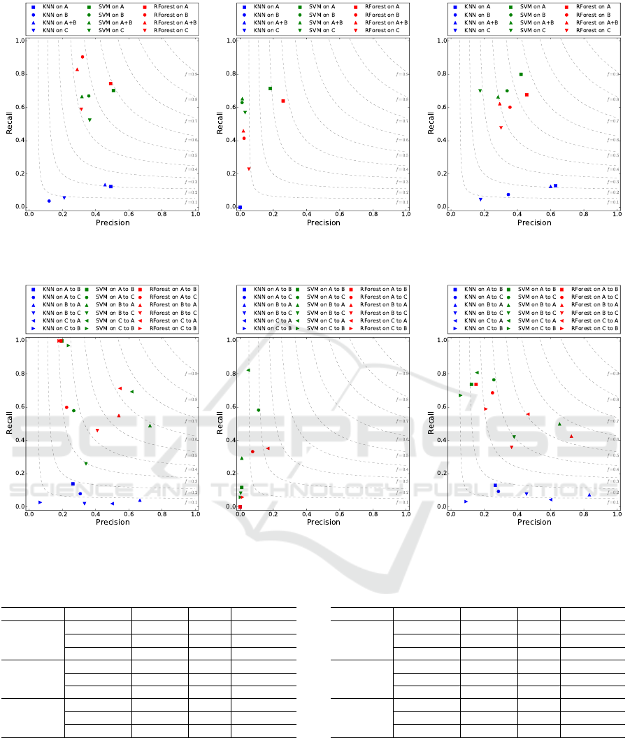
(a) Pass (b) Reception (c) Ball touch
Figure 5: Event recognition within data sets.
(a) Pass (b) Reception (c) Ball touch
Figure 6: Event recognition across data sets.
Table 2: Algorithms quality for prediction within data sets.
Algorithm Event Type Precision Recall F-Measure
KNN
pass 0.320 0.088 0.138
reception 0.000 0.000 0.000
ball touch 0.438 0.095 0.156
SVM
pass 0.387 0.641 0.483
reception 0.059 0.642 0.108
ball touch 0.305 0.716 0.428
RForest
pass 0.354 0.767 0.484
reception 0.089 0.436 0.148
ball touch 0.351 0.595 0.442
skills and players get exhausted over the period of a
match.
Finally, we aggregated the results for the predic-
tion across data sets, as explained in Section 5.2.
Since the precisions for the different event types are
nearly the same for the three algorithms (cf. Table
3), we used as a configuration for the aggregation a
Table 3: Algorithms quality for prediction across data sets.
Algorithm Event Type Precision Recall F-Measure
KNN
pass 0.356 0.055 0.095
reception 0.000 0.000 0.000
ball touch 0.422 0.076 0.128
SVM
pass 0.398 0.666 0.498
reception 0.031 0.327 0.057
ball touch 0.272 0.651 0.383
RForest
pass 0.311 0.727 0.435
reception 0.057 0.124 0.078
ball touch 0.373 0.544 0.443
weight of 3
−1
for every algorithm and a minimum
score of 2 · 3
−1
. Therefore, two out of three algo-
rithms have to find an event at a given timestamp, in
order to confirm this event. Table 4 shows that we
increased the f -measure for passes and ball touches
compared to all three algorithms between 1.6% and
41.9% (17.1% average). We also increased the f -
Recognizing Compound Events in Spatio-Temporal Football Data
33

measure for receptions compared to the KNN (6.7%)
and SVM (1%) algorithm, but decreased it about 1%
for RForest.
Table 4: Aggregation quality for prediction across data sets.
Event Type Precision Recall F-Measure
pass 0.426 0.647 0.514
reception 0.047 0.119 0.067
ball touch 0.372 0.713 0.489
To summarize, our results show that it is possi-
ble to detect football events from positional data with
our approach based on supervised learning. Also the
choice of a specific algorithm can have an extensive
impact on the quality of the predicted results. The
SVM and RForest algorithms showed reasonable re-
sults, whereas the KNN algorithm failed to convince
us for this use case. With the aggregation of the differ-
ent algorithms the results could be further improved.
Therefore, a valuable configuration of the weights and
the minimum score is needed. Nevertheless, there is
still potential for optimizations.
7 FUTURE WORK
In this section, we face issues discovered and suggest
proceedings to further improve and extend our work.
The missing z coordinate (height information) is nec-
essary to calculate features such as velocity, acceler-
ation and direction change correctly, since the ball is
moving in a three-dimensional space. When the ball
is out of bounds or the game has stopped the posi-
tional data should be ignored, because the data is in-
appropriate to draw conclusions about that. We also
discovered problems with the distinction of receptions
that occur directly before a pass, which happens when
a player receives the ball and immediately shoots it to
another player. A higher data resolution might help to
mitigate this issue.
To extend our approach it would be possible to
train the features for every player separately, since ev-
ery player has a different skill and shows its own be-
havior. It is also possible that a player changes its be-
havior between matches or even during a match, when
a player gets exhausted, or the teams adapt their tac-
tics to the game. This would make it even more chal-
lenging to classify the different event types. To val-
idate an event candidate it would be an extension to
integrate what is happening before and after the event
time and what the players around the event position
are doing. A good candidate to weight the features oc-
curing in a specific time window is the inter-quartile
range coverage algorithm (Schwarz et al., 2012a),
which is useful for detection of patterns with known
features in time-series data (Schwarz et al., 2012b).
We focused mainly on the moment of an event iden-
tified by the features of the ball, but probably more
information can be gathered this way.
8 CONCLUSION
In this paper, we proposed to detect events from po-
sitional data of football matches, in order to replace
the error-prone and time-consuming task of captur-
ing these events manually. We presented a super-
vised machine learning approach that classifies com-
pound football on the base of different features, which
are computed from positional data. To calculate
those features efficiently for over one million tracking
events per match, we used matrix operations, particu-
larly convolution, and optional GPU features to paral-
lelize and speedup the calculation. We used the Sup-
port Vector Machine, K-Nearest Neighbors and Ran-
dom Forest classification algorithms to recognize the
event classes of passes, receptions, shots on target and
clearances in our self-captured gold standard. Addi-
tionally, we enhanced the approach with a customiz-
able aggregation algorithm, to be able to weight the
outcome of the algorithms for different event types.
We evaluated the three algorithms by their qual-
ity of precision and recall. Compared to KNN algo-
rithm, the SVM and RForest algorithms showed rea-
sonable results with a precision of 31.1% up to 39.8%
and a recall of 66.6% up to 72.7% for passes. Recep-
tions seemed to be difficult to distinguish from passes
for the classification algorithms, which is why we re-
ceived lower results for them. We further improved
the results with the aggregation of the different algo-
rithms and increased the f -measures with an average
of 12.1% for all event types compared to the three
algorithms. To improve our approach for a practi-
cal use, we showed different ideas for future work.
In conclusion, our results showed that it is possible
to detect football events from positional data, but the
choice of a specific algorithm can have an extensive
impact on the quality of the predicted results.
REFERENCES
Altman, N. S. (1992). An introduction to kernel and nearest-
neighbor nonparametric regression. The American
Statistician, 46(3):175–185.
Anguita, D., Ghio, A., Oneto, L., Parra, X., and Reyes-
Ortiz, J. L. (2012). Human activity recognition
IoTBD 2016 - International Conference on Internet of Things and Big Data
34

on smartphones using a multiclass hardware-friendly
support vector machine. In Ambient assisted living
and home care, pages 216–223. Springer.
Barnard, M., Odobez, J.-M., and Bengio, S. (2003). Multi-
modal audio-visual event recognition for football
analysis. In Neural Networks for Signal Processing,
2003. NNSP’03. 2003 IEEE 13th Workshop on, pages
469–478. IEEE.
Beetz, M., von Hoyningen-Huene, N., Kirchlechner, B.,
Gedikli, S., Siles, F., Durus, M., and Lames, M.
(2009). Aspogamo: Automated sports game analysis
models. International Journal of Computer Science in
Sport, 8(1):1–21.
Bergstra, J., Breuleux, O., Bastien, F., Lamblin, P., Pascanu,
R., Desjardins, G., Turian, J., Warde-Farley, D., and
Bengio, Y. (2010). Theano: A CPU and GPU Math
Compiler in Python. In Proceedings of the Python for
Scientific Computing Conference (SciPy), 9.
Breiman, L. (2001). Random forests. Machine Learning,
45(1):5–32.
Carling, C., Williams, A. M., and Reilly, T. (2005). Hand-
book of soccer match analysis: A systematic approach
to improving performance. Psychology Press.
Christopher Mutschler, Holger Ziekow, and Zbigniew
Jerzak (2013). The DEBS 2013 Grand Challenge.
In ACM, editor, Proceedings of the 7th ACM Inter-
national Conference on Distributed Event-Based Sys-
tems, pages 289–294.
Connaghan, D., Kelly, P., O’Connor, N. E., Gaffney, M.,
Walsh, M., and O’Mathuna, C. (2011). Multi-sensor
classification of tennis strokes. In Sensors, 2011
IEEE, pages 1437–1440. IEEE.
Cortes, C. and Vapnik, V. (1995). Support-vector networks.
Machine Learning, 20(3):273–297.
Gal, A., Keren, S., Sondak, M., Weidlich, M., Blom, H., and
Bockermann, C. (2013). Grand challenge: The tech-
niball system. In Proceedings of the 7th ACM interna-
tional conference on Distributed event-based systems,
pages 319–324. ACM.
Horton, M., Gudmundsson, J., Chawla, S., and Es-
tephan, J. (2014). Classification of passes in foot-
ball matches using spatiotemporal data. arXiv preprint
arXiv:1407.5093.
Jiang, W. and Yin, Z. (2015). Human activity recognition
using wearable sensors by deep convolutional neural
networks. In Proceedings of the 23rd Annual ACM
Conference on Multimedia Conference, pages 1307–
1310. ACM.
Kautz, T., Groh, B. H., and Eskofier, B. M. (2015). Sensor
fusion for multi-player activity recognition in game
sports.
Mackenzie, R. and Cushion, C. (2013). Performance
analysis in football: A critical review and implica-
tions for future research. Journal of Sports Sciences,
31(6):639–676.
Madsen, K. G. S., Su, L., and Zhou, Y. (2013). Grand chal-
lenge: Mapreduce-style processing of fast sensor data.
In Proceedings of the 7th ACM international confer-
ence on Distributed event-based systems, pages 313–
318. ACM.
Pedregosa, F., Varoquaux, G., Gramfort, A., Michel, V.,
Thirion, B., Grisel, O., Blondel, M., Prettenhofer, P.,
Weiss, R., Dubourg, V., Vanderplas, J., Passos, A.,
Cournapeau, D., Brucher, M., Perrot, M., and Duch-
esnay, E. (2011). Scikit-learn: Machine Learning
in Python. Journal of Machine Learning Research,
12:2825–2830.
Peterek, T., Penhaker, M., Gajdo
ˇ
s, P., and Dohn
´
alek, P.
(2014). Comparison of classification algorithms for
physical activity recognition. In Innovations in Bio-
inspired Computing and Applications, pages 123–131.
Springer.
Schuldhaus, D., Zwick, C., K
¨
orger, H., Dorschky, E., Kirk,
R., and Eskofier, B. M. (2015). Inertial sensor-based
approach for shot/pass classification during a soccer
match.
Schwarz, C., Leupold, F., and Schubotz, T. (2012a). Short-
Term Energy Pattern Detection of Manufacturing Ma-
chines with In-Memory Databases - A Case Study.
In ENERGY 2012: The Second International Confer-
ence on Smart Grids, Green Communications and IT
Energy-aware Technologies, pages 7–12.
Schwarz, C., Leupold, F., Schubotz, T., Januschowski, T.,
and Plattner, H. (2012b). Rapid Energy Consumption
Pattern Detection with In-Memory Technology. Inter-
national Journal on Advances in Intelligent Systems,
5:415–426.
von der Gr
¨
un, T., Franke, N., Wolf, D., Witt, N., and Eid-
loth, A. (2011). A real-time tracking system for foot-
ball match and training analysis. In Microelectronic
systems, pages 199–212. Springer.
Recognizing Compound Events in Spatio-Temporal Football Data
35