House Price Estimation from Visual and Textual Features

Eman H. Ahmed and Mohamed Moustafa

Computer Science and Engineering Department, The American University in Cairo, Road 90, New Cairo, Cairo, Egypt

Keywords:

Support Vector Regression, Neural Networks, House Price Estimation, Houses Dataset.

Abstract:

Most existing automatic house price estimation systems rely only on some textual data like its neighborhood

area and the number of rooms. The ﬁnal price is estimated by a human agent who visits the house and assesses

it visually. In this paper, we propose extracting visual features from house photographs and combining them

with the house’s textual information. The combined features are fed to a fully connected multilayer Neural

Network (NN) that estimates the house price as its single output. To train and evaluate our network, we have

collected the ﬁrst houses dataset (to our knowledge) that combines both images and textual attributes. The

dataset is composed of 535 sample houses from the state of California, USA. Our experiments showed that

adding the visual features increased the R-value by a factor of 3 and decreased the Mean Square Error (MSE)

by one order of magnitude compared with textual-only features. Additionally, when trained on the textual-only

features housing dataset (Lichman, 2013), our proposed NN still outperformed the existing model published

results (Khamis and Kamarudin, 2014).

1 INTRODUCTION

Housing market plays a signiﬁcant role in shaping the

economy. Housing renovation and construction boost

the economy by increasing the house sales rate, em-

ployment and expenditures. It also affects the demand

for other relevant industries such as the construction

supplies and the household durables (Li et al., 2011).

The value of the asset portfolio for households whose

house is their largest single asset is highly affected

by the oscillation of the house prices. Recent stud-

ies show that the house market affects the ﬁnancial

institutions proﬁtability which in turn affects the sur-

rounding ﬁnancial system. Moreover, the housing

sector acts as a vital indicator of both the economy’s

real sector and the assets prices which help forecast

inﬂation and output (Li et al., 2011). The traditional

tedious price prediction process is based on the sales

price comparison and the cost which is unreliable and

lacks an accepted standard and a certiﬁcation pro-

cess (Khamis and Kamarudin, 2014). Therefore, a

precise automatic prediction for the houses’ prices is

needed to help policy makers to better design poli-

cies and control inﬂation and also help individuals for

wise investment plans (Li et al., 2011). Predicting the

houses’ prices is a very difﬁcult task due to the illiq-

uidity and heterogeneity in both the physical and the

geographical perspectives of the houses market. Also,

there is a subtle interaction between the house price

and some other macroeconomic factors that makes the

process of prediction very complicated. Some previ-

ous studies were conducted to search the most impor-

tant factors that affect the houses’ price. All the pre-

vious work was directed towards the textual attributes

of the houses (Khamis and Kamarudin, 2014; Ng and

Deisenroth, 2015; Park and Bae, 2015). So, we de-

cided to combine both visual and textual attributes

to be used in the price estimation process. Accord-

ing to (Limsombunc et al., 2004), the house price

gets affected by some factors like its neighbourhood,

area, the number of bedrooms and bathrooms. The

more bedrooms and bathrooms the house has, and the

higher its price. Therefore, we depended on these fac-

tors besides the images of the house to estimate the

price. The contribution of this paper:

• We provide the ﬁrst houses dataset, to our knowl-

edge, that combines both visual and textual at-

tributes to be used for price estimation. The

dataset will be publicly available for research pur-

poses.

• We propose a multilayer neural network for house

price estimation from visual and textual features.

We report the results of this proposed model using

the newly created benchmark dataset. Addition-

ally, we show that our model surpasses the state

of the art models, when tested using only the tex-

tual features, on an existing benchmark housing

H. Ahmed E. and Moustafa M.

House Price Estimation from Visual and Textual Features.

DOI: 10.5220/0006040700620068

In Proceedings of the 8th International Joint Conference on Computational Intelligence (IJCCI 2016), pages 62-68

ISBN: 978-989-758-201-1

dataset (Lichman, 2013). Our model also outper-

forms Support Vector Regression machine (SVR)

when trained and tested on our dataset.

The remaining of this paper is organized as follows:

we start by reviewing related work, followed by a

description of our newly created dataset. We then

present our proposed baseline NN model. The ex-

perimental results section demonstrates the accuracy

of our proposed model. Finally, we close with some

concluding remarks.

2 RELATED WORK

During the last decade, some work has been done

to automate the real estate price evaluation process.

The successes were in emphasizing the attributes of

the property such as the property site, property qual-

ity, environment and location. Comparing different

methods, we found that the previous approaches can

be classiﬁed into two main categories: Data disag-

gregation based models and Data aggregation based

models. The Data disaggregation based models try to

predict the house’s price with respect to each attribute

alone like the Hedonic Price Theory. However, The

Data aggregation models depend on all the house’s

attributes to estimate its price such as the Neural Net-

work and regression models. As an example of the

Data disaggregation models, the Hedonic Price The-

ory where the price of the real estate is a function of

its attributes. The attributes associated with the real

estate deﬁne a set of implicit prices. The marginal

implicit values of the attributes are obtained by dif-

ferentiating the hedonic price function with respect to

each attribute (Limsombunc et al., 2004). The prob-

lem with this method is that it does not consider the

differences between different properties in the same

geographical area. That’s why it is considered unre-

alistic. Flitcher et al in (Fletcher et al., 2000) tried

to explore the best way to estimate the property price

comparing the results of aggregation and disaggrega-

tion of data. They found that the results of aggre-

gation are more accurate. They also found that the

hedonic price of some coefﬁcients for some attributes

are not stable, as they change according to location,

age and property type. Therefore, they realized that

the Hedonic analysis can be effective while analysing

these changes but not for estimating the price based

on each attribute alone. Additionally, they discovered

that the geographical location of the property plays an

important role in inﬂuencing the price of the property.

For the Data aggregation model, Neural Network is

the most common model. Bin Khamis in (Khamis

and Kamarudin, 2014) compared the performance of

the Neural Network against the Multiple-Linear Re-

gression (MLR). NN achieved a higher R

value and

a lower MSE than the MLR. Comparing the results of

the Hedonic model versus the neural network model,

the neural network outperforms the Hedonic model by

achieving a higher R

value by 45.348% and a lower

MSE by 48.8441%. The lack of information in the

Hedonic model may be the cause of the poor perfor-

mance. However, there are some limitations in the

Neural Network Model, as the estimated price is not

the actual price but it is close to the real one. This

is because of the difﬁculty in obtaining the real data

from the market. Also, the time effect plays an im-

portant role in the estimation process which Neural

Networks cannot handle automatically. This implies

that the property price is affected by many other eco-

nomic factors that are hard to be included in the esti-

mation process. In this paper, we want to investigate

the impact of aggregating visual features with textual

attributes on the estimation process. Two estimation

models will be examined: the SVR and the NN.

3 DATASET DESCRIPTION

The collected dataset is composed of 535 sample

houses from California State in the United State. Each

house is represented by both visual and textual data.

The visual data is a set of 4 images for the frontal im-

age of the house, the bedroom, the kitchen and the

bathroom as shown in ﬁgure 1. The textual data rep-

resent the physical attributes of the house such as the

number of bedrooms, the number of bathrooms, the

area of the house and the zip code for the place where

the house is located. This dataset was collected and

annotated manually from publicly available informa-

tion on websites that sell houses. There are no re-

peated data nor missing ones. The house price in

the dataset ranges from $22,000 to $5,858,000. Table

1 contains some statistical details about our dataset.

This dataset is publicly available for further research

on (H.Ahmed, 2016).

Figure 1: Sample house from (realtor.com, 2016), where it

is represented by 4 images for the frontal side, the kitchen,

the bedroom and the bathroom.

House Price Estimation from Visual and Textual Features

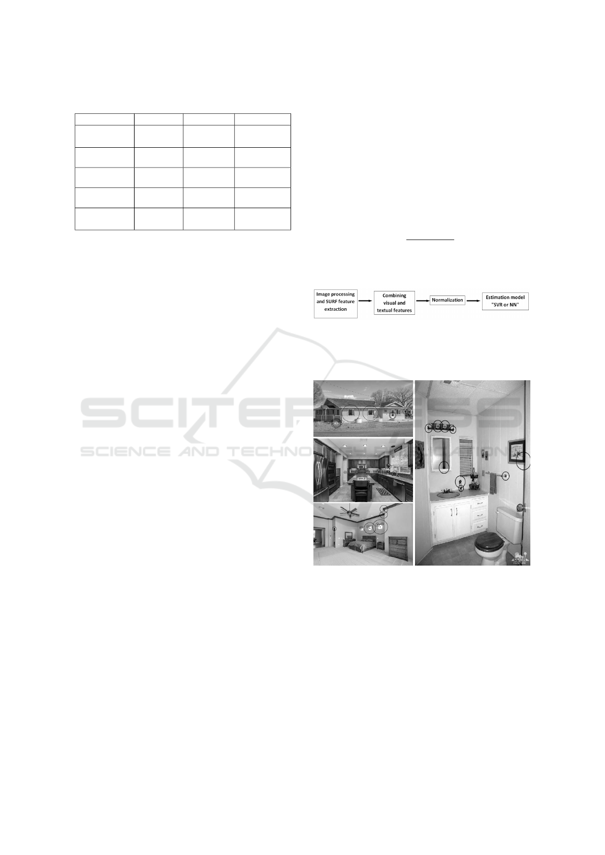
Table 1: Some details about our benchmark houses dataset.

Detail Average Minimum Maximum

House price

(USD) $589,360 $22,000 $5,858,000

House area

(sq. ft.) 2364.9 701 9583

Number of

bedrooms 3.38 1 10

Number of

bathrooms 2.67 1 7

Images

resolution 801x560 250x187 1484x1484

4 PROPOSED BASELINE

SYSTEM

The main aim of our research is to test the impact

of including visual features of houses to be used

for the houses’ prices estimation. Also, we tried to

ﬁnd the relationship between the number visual fea-

tures and the accuracy of the estimation using Support

Vector Regression and Neural Networks Model. As

shown in ﬁgure 2, our system has different processing

stages, each of them is represented by a module block.

The ﬁrst module in our system is image processing

where the histogram equalization technique (Kapoor

and Arora, 2015) is used to increase the global con-

trast of the dataset images. This technique resulted

in better distribution of the color intensity among all

the images and allowed the areas of lower local con-

trast to gain high contrast by effectively spreading

out the most frequent intensity values. After that,

the Speeded Up Robust Features (SURF) extractor

(Bay et al., 2008) is used for to extract the visual fea-

tures from the images. SURF uses an integer approx-

imation of the determinant of Hessian blob detector,

which can be computed with 3 integer operations us-

ing a precomputed integral image. Its feature descrip-

tor is based on the sum of the Haar wavelet response

around the point of interest. These can also be com-

puted with the aid of the integral image (Bay et al.,

2008). In this step, the strongest n features were ex-

tracted from each image of the house, then these fea-

tures were concatenated together in a vector format

along with the textual attributes of the same house in

a speciﬁc order to represent the total features of this

house. Figure 3 is an example for the extracted SURF

features from the 4 images of a house in the dataset.

The extracted features emphasize corners, sharp tran-

sitions and edges. It was found visually that these fea-

tures mark interest points in the images as shown in

the frontal image of the house, where the windows

were selected as important features. The value for

the extracted features n varied from one experiment

to another as will be explained in section 5. SURF

feature extractor produced better results compared to

the Scale Invariant Feature Transform (SIFT) extrac-

tor (Lowe, 2004) and it was also faster therefore, it

was used in all of our experiments. In the last mod-

ule, the aggregated features are passed to one of the

estimation modules: either the SVR or the NN after

normalization. Normalization is a preprocessing tech-

nique where data is scaled between the range of 0 and

1. The formula used for normalization is:

−min(x)

max(x)−min(x)

(1)

Where x = (x

, ..., x

) and z

is the i

normalized data

point.

Figure 2: Proposed system processing pipeline.

Each estimation model has its own architecture

and parameters.

Figure 3: Example for the extracted SURF features from

the dataset.

4.1 Support Vector Regression (SVR)

Support Vector Machines are Machine Learning ap-

proaches for solving multi-dimensional function es-

timation and regression problems. SVMs are de-

rived from the statistical learning theory and they

are based on the principle of optimal separation of

classes. SVMs use high dimensional feature space to

learn and yield prediction functions that are expanded

on a subset of support vectors (Basak et al., 2007).

There are two main categories for the SVMs: Support

NCTA 2016 - 8th International Conference on Neural Computation Theory and Applications

Vector Classiﬁcation (SVC) and Support Vector Re-

gression (SVR). In SVCs, the SVMs try to separate

the classes with the minimum generalization error if

the classes are separable. If the classes are not seper-

able, SVMs try to get the hyperplane that maximizes

the margin and reduces the misclassiﬁcation error. In

SVRs, Vapnik in (Sain, 1996) introduced an alterna-

tive intensive loss function ε that allows the margin

to be used for regression. The main goal of the SVR

is to ﬁnd a function f (x) that has at most ε deviation

from the actually obtained targets for all the training

data and at the same time as ﬂat as possible. In other

words, the error of the training data has to be less

than ε that is why the SVR depends only on a subset

of the training data because the cost function ignores

any training data that is close or within ε to the model

prediction (Deswal and Pal, 2015; Basak et al., 2007).

A deep explanation of the underlying mathematics of

the SVR is given in (Basak et al., 2007). It also points

out that the SVR requires a careful selection of the

kernel function type and the regularization parameter

(C). The kernel function can efﬁciently perform non-

linear regression by implicitly mapping the inputs into

a higher dimensional feature space to make it possi-

ble to perform linear regression. The (C) parameter

determines the trade-off between the ﬂatness of the

function and the amount by which the deviations to

the error more than ε can be tolerated (Deswal and

Pal, 2015). In our experiments, the Histogram Inter-

section Kernel was chosen as the kernel type and the

optimal value for the parameter (C) was obtained after

several experiments on the dataset to obtain the best

result. Histogram Intersection is a technique proposed

in (Swain and Ballard, 1991) for color indexing with

application to object recognition and it was proven in

(Barla et al., 2003) that it can be used as a kernel for

the SVM as an effective representation of color-based

recognition systems that are stable to occlusion and to

change of view.

The metrics for evaluating the performance of the

SVR are the coefﬁcient of determination (R

) and the

Mean Squared Error (MSE).

4.2 Neural Networks (NNs)

Neural Networks are artiﬁcial intelligence models

that are designed to replicate the human brain. NNs

typically consist of layers as shown in ﬁgure 4 .These

layers are formed by interconnected processing units

called neurons where the input information is pro-

cessed. Each neuron in a layer is connected to the

neurons in the next layer via a weighted connection.

This weighted connection W

i j

is an indication of the

strength between node i where it is coming from

and node j where it is going. A three layer NN is

shown in ﬁgure 4. The structure of the NN is an in-

put layer, one or more hidden layers and an output

layer. Hidden layers can be called as feature detec-

tors because the activity pattern in the hidden layer is

an encoding of what the network thinks are the sig-

niﬁcant features of the inputs. When combining the

hidden layers features together, the output unit can

perform more complex classiﬁcation/regression tasks

and solve non-linear problems. NNs that have one

or more hidden layers are used for solving non-linear

problems. The architecture of the NN depends on the

complexity of the problem.

Figure 4: General structure of the Neural Network where

it consists of 3 layers: the input layer, one hidden layer of 4

neurons and the output layer.

Each neuron performs a dot product between the

inputs and the weights and then it applies an activa-

tion function. There are many different types of acti-

vation functions. The most common activation func-

tion that is also used in our experiments is the sigmoid

activation function f (x) =

1+e

−x

. The advantage of

this function is that it is easy to differentiate which

dramatically reduces the computation burden in the

training. Both the inputs and the outputs of the sig-

moid function are in the range between 0 and 1 that is

why we had to normalize the data before starting the

NN. Our NN was trained using Levenberg–Marquardt

algorithm (LMA) (Gavin, 2011) which is a tech-

nique used to solve non-linear least square problems.

The Levenberg-Marquardt method is a combination

of two minimization methods: the gradient descent

method and the Gauss-Newton method. In the gradi-

ent descent method, the sum of the squared errors is

reduced by updating the parameters in the steepest-

House Price Estimation from Visual and Textual Features

descent direction. In the Gauss-Newton method, the

sum of the squared errors is reduced by assuming the

least squares function is locally quadratic, and ﬁnd-

ing the minimum of the quadratic. The Levenberg-

Marquardt method acts more like a gradient-descent

method when the parameters are far from their op-

timal value, and acts more like the Gauss-Newton

method when the parameters are close to their opti-

mal value. We used coefﬁcient of determination (R

)

and the Mean Squared Error (MSE) for evaluating the

performance of the NN on our dataset and to compare

the results with the (Lichman, 2013) housing dataset

4.3 Performance Evaluation

4.3.1 Mean Square Error

Mean Square Error is a measure for how close the

estimation is relative to the actual data. It measures

the average of the square of the errors deviation of the

estimated values with respect to the actual values. It

is measured by:

MSE =

∑

i=1

( ˆy − y)

(2)

where ˆy is the estimated value from the regression and

y is the actual value. The lower the MSE, the better

the estimation model.

4.3.2 The Coefﬁcient of Determination R

The coefﬁcient of determination is a measure of the

closeness of the predicted model relative to the actual

model. It is calculated a set of various errors:

SSE =

∑

i=1

( ˆy

− y

)

(3)

SST =

∑

i=1

( ¯y − y

)

(4)

SSE is the Sum of Squares of Error and SST is the

Sum of Squares Total. The R-squared value is calcu-

lated by:

= 1 −

SSE

SST

(5)

The value of R

ranges between 0 and 1, the higher

the value, the more accurate the estimation model.

5 EXPERIMENTS AND RESULTS

In this section, we will describe the experiments we

have done in both estimation models: SVR and NN

and compare the NN with the (Lichman, 2013) Hous-

ing dataset.

5.1 SVR Experiments

In the SVR model, 428 houses were used for training

which is 80% of the dataset and 107 houses were used

for testing which is 20% of the dataset. The SVR was

trained and tested on different number of the extracted

SURF features each time to ﬁnd the relationship be-

tween the number of features and the accuracy of the

estimation model. 16 different cases were tested start-

ing with training and testing with the textual attributes

only with no visual features and moving forward to

extracting more SURF features up to 15. In our exper-

iments, the Histogram Intersection Kernel was cho-

sen as the kernel type and the optimal value for the

parameter (C) was obtained after several experiments

on the dataset to obtain the best result. Figures 6 and

7 in section 5.2 show that performance of the SVR in-

creases with adding more visual features till it reaches

9 visual features where the model achieves the lowest

MSE value of 0.0037665 and the highest R −Value of

0.78602. Then, the SVR performance started to dete-

riorate gradually after reaching its highest point at 9

features.

5.2 Neural Networks Experiments

As shown in ﬁgure 4, we adopted a fully connected

architecture with one 4-units hidden layer. The prob-

lem was expected to be non-linear that is why the

networks has hidden layers. The number of hidden

nodes was chosen to be somewhere between the num-

ber of input nodes and output nodes and by trying dif-

ferent number of neurons in the hidden layer, it was

proven that having 4 neurons is the optimal architec-

ture. Our neurons had sigmoid activation function and

trained with the Levenberg Marquardt variation of the

error-back-propagation technique. This architecture

produced the best results during our experiments. We

divided our dataset into three pieces: 70% for train-

ing, 15% for validation, and 15% for testing. To

avoid over-ﬁtting, we have stopped the training after

5 epochs, a measure of the number of times all of the

training vectors are used once to update the weights,

because the validation error started to increase. Figure

5 shows the performance of the Network highlighting

the training, validation and test MSEs and when the

training process was stopped to avoid over-ﬁtting.

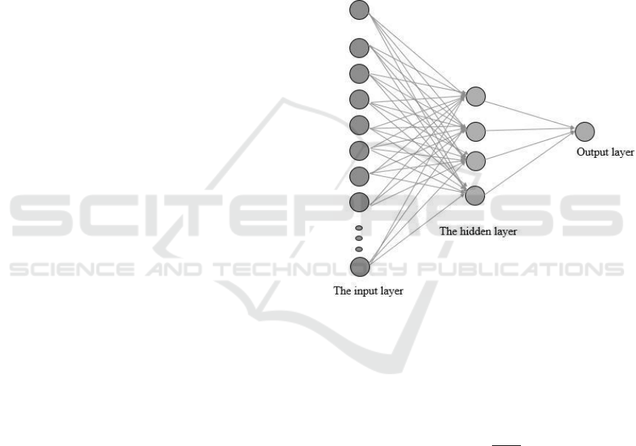
Figures 6 and 7 show that combining 4 SURF fea-

tures with the textual attributes results in achieving

the highest R−Value of 0.95053 and the least MSE of

0.000959. In the NN model, the MSE starts very high

with no visual features and with increasing the vi-

sual features, the MSE starts to decrease till it reaches

its minimum value at 4 features, and then it gradu-

NCTA 2016 - 8th International Conference on Neural Computation Theory and Applications

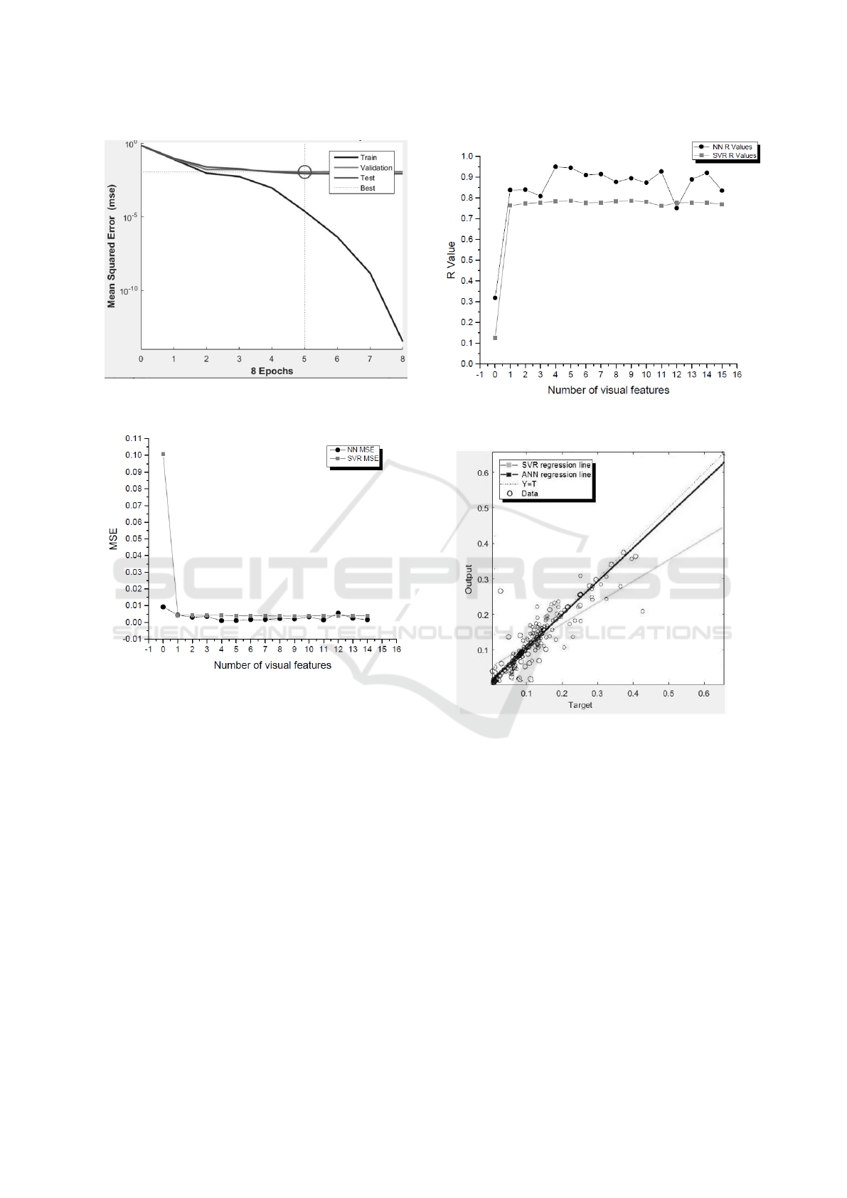
Figure 5: Performance graph shows the MSE of the net-

work per epoch on training, validation and testing sets.

Figure 6: The relationship between the number of features

and the MSE in the NN model and the SVR model.

ally starts to increase till 16. Figure 6 shows that the

NN outperforms the SVR model by achieving a lower

MSE by 76.02%. Also, ﬁgure 7 shows that the NN

achieved a higher R −Value by 21.05% than the SVR.

Also ﬁgure 8 shows that the regression line produced

by the NN is more accurate because the estimated val-

ues are much closer to the actual data.

5.3 Our NN Model on (Lichman, 2013)

Housing Dataset

To rule out data dependency, we have tested our

model on the (Lichman, 2013) benchmark hous-

ing dataset that has 506 houses, each with 13 tex-

tual attributes such as average number of rooms per

dwelling, age of the house, full-value property tax,

etc. We compared our results with (Khamis and Ka-

marudin, 2014) model that used NN to estimate the

Figure 7: The relationship between the number of features

and the R-Value in the NN model and the SVR model.

Figure 8: The regression line for the SVR and the NN.

house price based on textual features only. We repli-

cated their model to be able to compare the results of

both training and testing instead of the training only

which was reported in the paper. We compared the

MSE and R − Value in both training and testing and

our model outperforms their model. Average prices

were used while calculating the MSE to compare the

results with (Lichman, 2013) model that is why the

MSE values are larger than the values reported on our

dataset.

The results tabulated in table 2 show that our

model achieves an MSE of 9.708× 10

and R −Value

of 0.9348 on the testing set which is better that Bin

Khamis’s model that achieves an MSE of 1.713× 10

and R-Value of 0.87392. Our model achieves a lower

MSE on the training set by 99.54% and on the testing

set by 99.43%. It also achieves a higher R − Value by

House Price Estimation from Visual and Textual Features

Table 2: Comparison between our NN performance and Bin

Khamis’s model.

Training

MSE

Training

R-Value

Testing

MSE

Testing

R-Value

Bin Khamis’s

model 1.293 E9 0.9039 1.713 E9 0.87392

Our

model 5.9223 E6 0.96537 9.708 E6 0.9348

6.8% on the training set and on the testing set 6.97%.

These results show that our Neural Network model

does not depend on our own dataset.

6 CONCLUSION

This paper announces the ﬁrst dataset, to our knowl-

edge, that combines both visual and textual features

for house price estimation. Other researchers are in-

vited to use the new dataset as well. Through experi-

ments, it was shown that aggregating both visual and

textual information yielded better estimation accuracy

compared to textual features alone. Moreover, better

results were achieved using NN over SVM given the

same dataset. Additionally, we demonstrated empir-

ically that the house price estimation accuracy is di-

rectly proportional with the number of visual features

up to some level, where it barely saturated. We be-

lieve this optimal number of features depends on the

images content. We are currently studying the rela-

tionship of the image content to the optimal number

of features. In the near future, we are planning to ap-

ply deeper neural networks to extract its own features

as well as trying other visual feature descriptors, e.g.,

Local Binary Patterns (LBP).

REFERENCES

Barla, A., Odone, F., and Verri, A. (2003). Histogram in-

tersection kernel for image classiﬁcation. In Image

Processing, 2003. ICIP 2003. Proceedings. 2003 In-

ternational Conference on, volume 3, pages III–513–

16 vol.2.

Basak, D., Pal, S., and Patranabis, D. C. (2007). Support

vector regression. Neural Information Processing-

Letters and Reviews, 11(10):203–224.

Bay, H., Ess, A., Tuytelaars, T., and Van Gool, L. (2008).

Speeded-up robust features (SURF). Computer vision

and image understanding, 110(3):346–359.

Deswal, S. and Pal, M. (2015). Comparison of Polyno-

mial and Radial Basis Kernel Functions based SVR

and MLR in Modeling Mass Transfer by Vertical and

Inclined Multiple Plunging Jets. International Jour-

nal of Civil, Environmental, Structural, Construction

and Architectural Engineering, (9):1214 – 1218.

Fletcher, M., Gallimore, P., and Mangan, J. (2000). The

modelling of housing submarkets. Journal of Property

Investment & Finance, 18(4):473–487.

Gavin, H. (2011). The Levenberg-Marquardt method for

nonlinear least squares curve-ﬁtting problems. De-

partment of Civil and Environmental Engineering,

Duke University, pages 1–15.

H.Ahmed, E. (2016). Houses dataset.

https://github.com/emanhamed/Houses-dataset.

Kapoor, K. and Arora, S. (2015). Colour image enhance-

ment based on histogram equalization. Electrical

& Computer Engineering: An International Journal,

4(3):73–82.

Khamis and Kamarudin (2014). Comparative Study On Es-

timate House Price Using Statistical And Neural Net-

work Model .

Li, Y., Leatham, D. J., et al. (2011). Forecasting Housing

Prices: Dynamic Factor Model versus LBVAR Model.

Lichman, M. (2013). UCI Machine Learning Repository.

Limsombunc, V., Gan, C., and Lee, M. (2004). House Price

Prediction: Hedonic Price Model vs. Artiﬁcial Neu-

ral Network. American Journal of Applied Sciences,

1(3):193–201.

Lowe, D. G. (2004). Distinctive image features from scale-

invariant keypoints. International journal of computer

vision, 60(2):91–110.

Ng, A. and Deisenroth, M. (2015). Machine learning for a

london housing price prediction mobile application.

Park, B. and Bae, J. K. (2015). Using machine learning

algorithms for housing price prediction: The case of

fairfax county, virginia housing data. Expert Systems

with Applications, 42(6):2928 – 2934.

realtor.com (2016). real estate agent website.

Sain, S. R. (1996). The nature of statistical learning theory.

Technometrics, 38(4):409–409.

Swain, M. J. and Ballard, D. H. (1991). Color indexing. In-

ternational Journal of Computer Vision, 7(1):11–32.

NCTA 2016 - 8th International Conference on Neural Computation Theory and Applications