Bark Recognition to Improve Leaf-based Classiﬁcation in Didactic Tree

Species Identiﬁcation

Sarah Bertrand

, Guillaume Cerutti

and Laure Tougne

Univ. Lyon, Lyon 2, LIRIS, F-69676 Lyon, France

INRIA, Virtual Plants INRIA Team, Montpellier, France

Keywords:

Bark, Leaf, Tree Recognition, Smart-phone.

Abstract:

In this paper, we propose a botanical approach for tree species classiﬁcation through automatic bark analysis.

The proposed method is based on speciﬁc descriptors inspired by the characterization keys used by botanists,

from visual bark texture criteria. The descriptors and the recognition system are developed in order to run on

a mobile device, without any network access. Our obtained results show a similar rate when compared to the

state of the art in tree species identiﬁcation from bark images with a small feature vector. Furthermore, we

also demonstrate that the consideration of the bark identiﬁcation signiﬁcantly improves the performance of

tree classiﬁcation based on leaf only.

1 INTRODUCTION

Nowadays, the growth of urbanization and techno-

logy has reduced the knowledge and uses of plants

by humans. However, the environment and its na-

tural resources are raising a growing concern. The

ability to identify the species of plants seems essen-

tial in the understanding of our green environment.

Thereby, providing an inexperienced person, who had

no knowledge in botany, with a tool to identify the

plants that surround him would be a great advance.

The portion of the population using a smart-

phone, incorporating a camera, a GPS, etc. grows in-

creasingly. These phones allow furthermore to down-

load additional applications with other functions than

communication. These smart-phones are ideal mate-

rials for applications related to image analysis.

From these two facts, let us consider the case

where a person, wandering through a forest or a city

park, wishes to recognize a species of tree. He then

takes a picture of the different organs of the plant

(leaf, bark, ﬂower) using his mobile phone. By

means of interactions between the smart-phone (via

the touch screen) and the user, and of course of treat-

ments and image processing, the system would return

a short list of species that may correspond to the plant

the user seeks to identify, coupled with a conﬁdence

rate.

Applications for smart-phone have been de-

veloped to address this subject, such as Leaf Snap

(Kumar et al., 2012), Pl@ntNet (Go

eau et al., 2013a),

or Folia (Cerutti et al., 2013). Furthermore, plant re-

cognition has recently been the subject of research in

the ﬁeld of image processing. Challenges have been

organized especially the ImageCLEF Challenge since

2011 (Go

eau et al., 2011).

Even though the leaves are the most used organs

for tree classiﬁcation in the applications, as they are

easily observed and described, the other parts of the

tree can help the recognition of tree species. In this

article, we focus on the recognition of tree species

through the bark. We choose to process this part of

the tree as it is always observable throughout the year

(not like ﬂowers or fruits), and can be easily photo-

graphed.

Since 2013, recognition of plants in the Image-

CLEF Challenge spread to other plant parts and not

only leaves as the 2011 and 2012 editions. In these

challenges, the different teams program algorithms in

order to recognize plant species through several im-

ages of the plant. In (Go

eau et al., 2013b) and (Go

eau

et al., 2014) we can see the evolution of the extracted

features used for the identiﬁcation of the bark. Un-

til 2014, the majority of the algorithms was based

on the detection and characterization of points such

as SIFT (Scale-invariant feature transform) (Lowe,

1999) or SURF (Speeded-Up Robust Features) (Bay

et al., 2006), with color information as well as in-

formation from Fourier transforms or LBP (local bin-

ary pattern) (Ojala et al., 1996), with bag-of-word ap-

Bertrand S., Cerutti G. and Tougne L.

Bark Recognition to Improve Leaf-based Classiﬁcation in Didactic Tree Species Identiﬁcation.

DOI: 10.5220/0006108504350442

In Proceedings of the 12th International Joint Conference on Computer Vision, Imaging and Computer Graphics Theory and Applications (VISIGRAPP 2017), pages 435-442

ISBN: 978-989-758-225-7

435

proaches. Texture descriptors were not used for the

bark recognition as they gave poorer results. Since the

ImageCLEF 2015 edition (Go

eau et al., 2015), there

is a large use of deep learning approaches, not only

for the classiﬁcation, but also for the features extrac-

tion. The GoogLeNet convolutional neural network

(Szegedy et al., 2015) has been employed by nearly

half of the teams. Only one team used hand-crafted

visual features.

These methods are efﬁcient but ﬁrst, they need

lots of training images, which is often hard to obtain

in the botanic domain. Secondly, they run as black

boxes that is to say they only give a classiﬁcation res-

ult without giving the user the possibility to under-

stand the result. But, the work that is proposed in this

article takes part of a pedagogic project the goal of

which is to learn the user to recognize a tree or a shrub

from its organ. For the leaves, a method based on

botanic criteria has already been developed by (Cer-

utti et al., 2013), which allows showing the user the

discriminant criteria during the recognition process.

The presented work aims at pursuing in this way us-

ing features the botanists use to discriminate the bark.

Notice also that as the goal is to do the image treat-

ment on smart-phones, as very often the Internet is

not reachable in the countryside, so we would like a

feature vector with reasonable size and, computation

time of it and classiﬁcation time in real time that is to

say in a few seconds.

In the following, we will present in part II the con-

struction of the features vector describing a bark im-

age. The next part III will display our different results

on the bark database and the improvement of the pro-

cessing of the bark on the tree species classiﬁcation

only based on the leaves.

2 BARK ANALYSIS

Our proposed method differs from the state of the

art in the sense that it is based on the extraction of

descriptors similar to those used by botanists from

visual texture criteria. More speciﬁcally, the method

simulates the bark recognition described by Michael

Wojtech in his book (Wojtech, 2011). In this ap-

proach, the barks are ﬁrst classiﬁed into different fam-

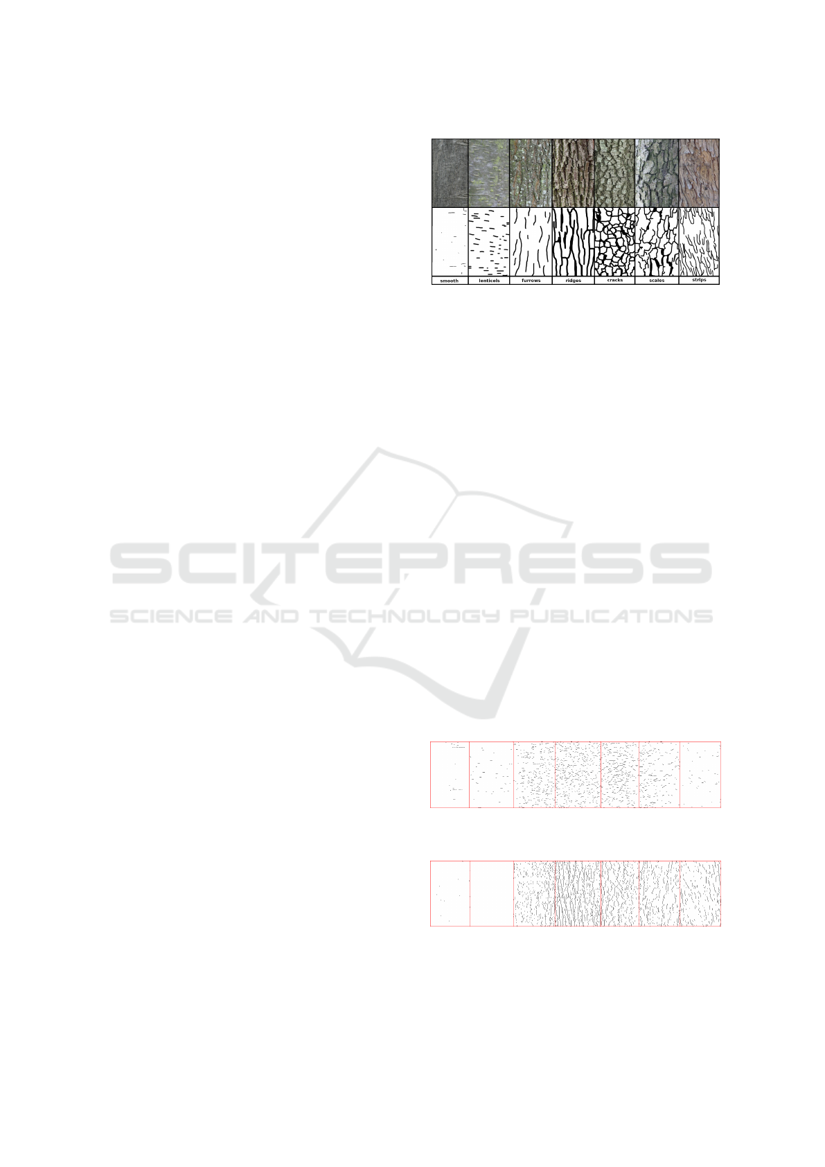
ilies as shown in Figure 1.

The ﬁrst row contains photos of characteristic bark

for each families. The second row highlights the dis-

tinctive bark structure of each photo of bark with a

drawing. More drawings can be found in (Wojtech,

2011). After identifying the type of bark, botanists

also take into account the color or other structural ele-

ments in order to recognize the tree species.

Figure 1: Different classes of bark structure based on visual

criteria.

In the following parts, we present the extracted

features to recognize the various types of barks and

then the different tree species.

2.1 Shape of the Bark

In this section, we propose a method to describe pre-

cisely the structure of the bark, not only whether it

has a vertical or horizontal structure. The goal is to

identify the different types of bark (Figure 1), i.e.,

bring out the forms (scales, straps, cracks, etc) of the

bark. For this, at ﬁrst, we need to extract the edges

of the shapes. For this purpose, we use the Canny al-

gorithm (Canny, 1986). Let us denote by M

and M

respectively the horizontal and the vertical maps ob-

tained with a horizontal ﬁlter F

and a vertical ﬁlter





−1 −2 −1

0 0 0

1 2 1





and F





−1 0 1

2 0 2

−1 0 1





(1)

The results of this Canny processing are visible on

Figure 2 for M

and on Figure 3 for M

Figure 2: Map of horizontal edges M

obtained from Figure

Figure 3: Map of vertical edges M

obtained from Figure

Using the maps of edges images, we can estimate

the dissimilarity between the different families of

VISAPP 2017 - International Conference on Computer Vision Theory and Applications

436

bark. To characterize the distribution of contours, we

propose to place a grid over the maps of edges images,

and to count the number of intersections between the

grid lines and the maps of contours. Speciﬁcally, from

(respectively M

), we focus on the intersections

between these contours and horizontal lines (vertical

respectively) grid. Then, for each row (column re-

spectively) grid, we calculate the number of intersec-

tions. This generates a ”vertical word” (respectively

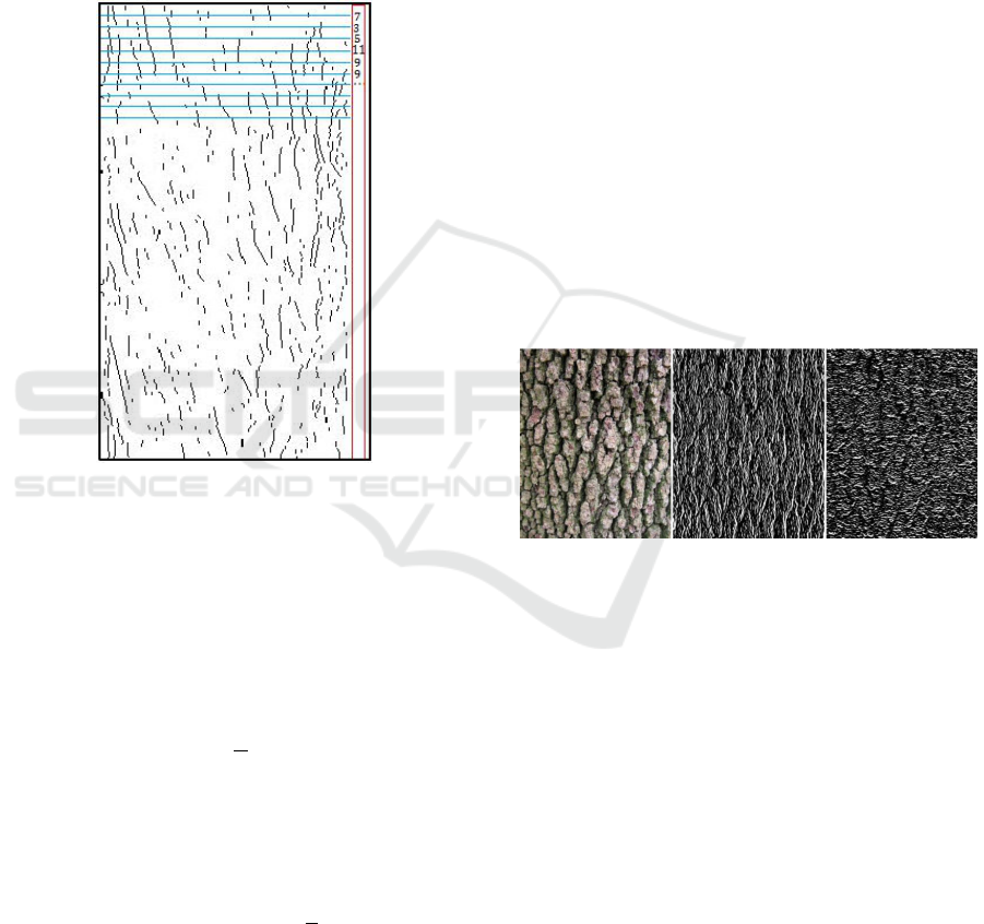
”horizontal word”) (see Figure 4).

Figure 4: Formation of the vertical word.

More formally, let l be the number of rows of

the image, c the number of columns, with λ

the fre-

quency of the vertical gridlines and λ

the frequency

of the horizontal grid. The higher the frequencies λ

and λ

, the higher the structure is precisely described.

The ”vertical word” W

is the concatenation of the in-

tersections v

with l varying from 0 to l with the fre-

quency of the grid λ

∑

c=0

l,c

(2)

with

(

l,c

= 1 if M

(λ

, λ

) = 1

l,c

= 0 else

(3)

and V =

{

}

0≤l≤

(4)

and M

are ﬁnally characterized by two

words, respectively W

and W

, that deﬁne the fre-

quency and distribution of the edges. If a word con-

tain mostly zeroes it means that the corresponding ori-

entation is rather smooth. When the ridges of the bark

are practically uninterrupted, the ”vertical word” will

be homogeneous. We will give in the Results section

some elements to explain the choice the discretization

steps in the two directions.

2.2 Bark Orientation

As we can see in Figure 1, barks may have structures

with different orientations, i.e. horizontal, horizontal

and/or vertical, or just be smooth. The orientation of

the bark is a recognition criterion. The image ﬁlter-

ing by Gabor wavelet can distinguish the direction

and frequency of the structure of the bark. Accord-

ing to Huang (Huang et al., 2006), only 6 orienta-

tions and 4 scales for the sinusoid forming the Gabor

wavelet are sufﬁcient to analyse the bark. However,

in the case of our application, the distance between

the smart-phone and the tree trunk may vary. Our

method must be scale independent as we can not con-

trol the camerawork. In addition, we want to determ-

ine, initially, whether the structure of the bark is ho-

rizontal or vertical, so only two orientations appears

adequate (0

◦

and 90

◦

). Figure 5 shows an example of

bark ﬁltered by two identical Gabor wavelets except

for the orientation.

Figure 5: Results of 0

◦

orientation Gabor ﬁltering (center)

and 90

◦

(right) of the initial image (left).

In order to have a characteristic vector of each

bark which is independent of the shooting distance,

we average four ﬁltered images by Gabor wavelets

with four different sinusoidal scales. The scales are

adjusted in order to highlight the horizontal and ver-

tical ridges of the bark, similarly to Figure 1.

The feature vector G reﬂecting the orientation of

the structure using Gabor ﬁlters consists of the mean

and the standard deviation of the ﬁltered image with

an orientation of 0

◦

, σ

and µ

, and the standard devi-

ation image ﬁltered at 90

◦

, σ

. We considered in-

cluding also the average of images at 90

◦

, but this

feature appeared as not discriminant, so we decided

to leave it apart, ending up with a simple feature vec-

tor of dimension 3: G : [σ

] . For the moment,

our features vector is composed of this Gabor vec-

tor and of W

and W

. We will show in the Results

section the positive contribution of the Gabor vector

concatenated with the two words W

and W

Bark Recognition to Improve Leaf-based Classiﬁcation in Didactic Tree Species Identiﬁcation

437

2.3 Bark Color

A second discriminant aspect for tree bark recog-

nition used by botanists is the color. Colorime-

tric descriptors were used in the challenge Image

CLEF 2013 by the teams showing the best results

(Bakic et al., 2013) (Nakayama, 2013). Several color

spaces were tested. We favored color spaces where

color channels were independent of brightness as the

descriptor should not be inﬂuenced by the presence of

shadows or by the changing of illumination that can

occur over the day and the year. The L* a* b* color

space seemed appropriate because of the channel a*

coding the red/green opposition and as we know the

bark of trees have brown, red, green, or gray shades.

However, the hue channel (H) of the HSV color space

was chosen because it gives us better classiﬁcation

results. It is because the hue channel can also man-

age the case of yellowish bark. The hue channel al-

lows to cover the whole range possible of bark color

with a single channel with 256 bins, contrary to the

concatenation of the a* and b* channels that would

have given a doubled size color feature vector. As a

reminder, we try to have a reasonable size feature vec-

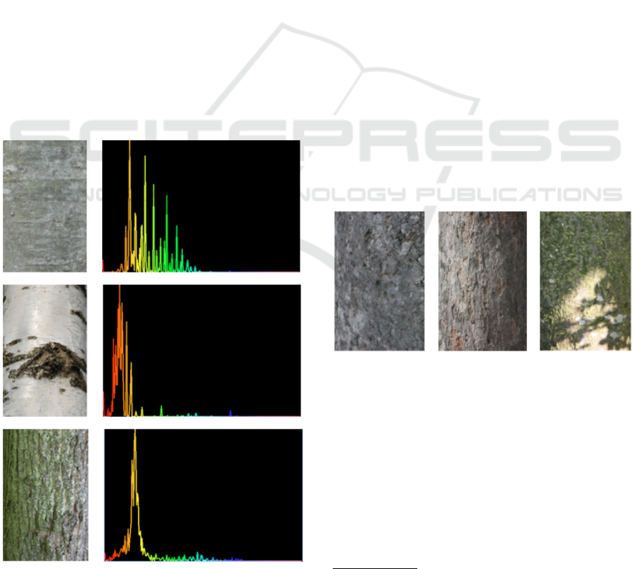
tor. Figure 6 shows the hue histogram for some bark

images.

Figure 6: Hue histogram for different barks.

Finally, the feature vector used for bark classiﬁc-

ation F

therefore consists in the concatenation of the

vector of Gabor G, W

and W

and the hue histogram

3 RESULTS

3.1 Bark Classiﬁcation

For the bark classiﬁcation, we have a database of 2559

bark image belonging to 101 tree species from the

data bank Pl@ntView

. Pictures of bark have the

same orientation as the tree (portrait mode). In our

practical application, we have re-sized these images

in order that the picture contain only the texture of

the bark, not the background, and no other elements

such as branch, leaves, or lichen. As a matter of

fact, we can make the assumption that the interface

of the application can guide the user to take such a

king of photos. However, we have kept the bark im-

ages which have a gradient of light or shadows (see

Figure7). This allows us to have an algorithm which

should work with images shot in non-optimal condi-

tions by beginners. We may also note that the number

of bark images is not the same for all the species (20

in average, but can go up to 100 for some species and

2 or 3 for others). The low number of samples for

some species makes it difﬁcult to train a performing

classiﬁer.

Figure 7: Bark of Acer Pseudoplatanus with homogeneous

luminosity, gradient of light or shadows.

As expressed in the introduction, we use a SVM

in order to classify the feature vector. The kernel

of the SVM is a Radial Basis Function (RBF) kernel

(Vapnik, 1999). We use a 1-vs-all algorithm, i.e. we

have one binary SVM for each species, with the class

species S versus the class non-S species. For each

query bark, we compute the feature vector then we

give this vector to all the 101 SVM classiﬁers. After-

wards the result is the species which the correspond-

ing classiﬁer gives the higher probability of afﬁliation

http://publish.plantnet-project.org/project/plantclef

VISAPP 2017 - International Conference on Computer Vision Theory and Applications

438

to the species S. On a Macbook Pro dating from 2011,

with a processor 2.7 GHz IntelCore i7 and a memory

4 GB 1333 MHz, we get a classiﬁcation result in less

than a second. As the last smart-phones have on aver-

age a processor of 2 GHz and quad-core, that make us

believe that our method could run on these devices.

Train is performed on half of the database, and

tests are performed on the second half. We obtain

a classiﬁcation rate equals to 30,7%. If we observe

the results of the plant task of the LifeCLEF chal-

lenges (Go

eau et al., 2015), plant recognition via the

stem gives the worst classiﬁcation rate compared to

the other other organs. The state of the art give around

30% of good identiﬁcation. So, with our method, we

achieve the same level with a quite short feature vec-

tor and without heavy classiﬁcation process.

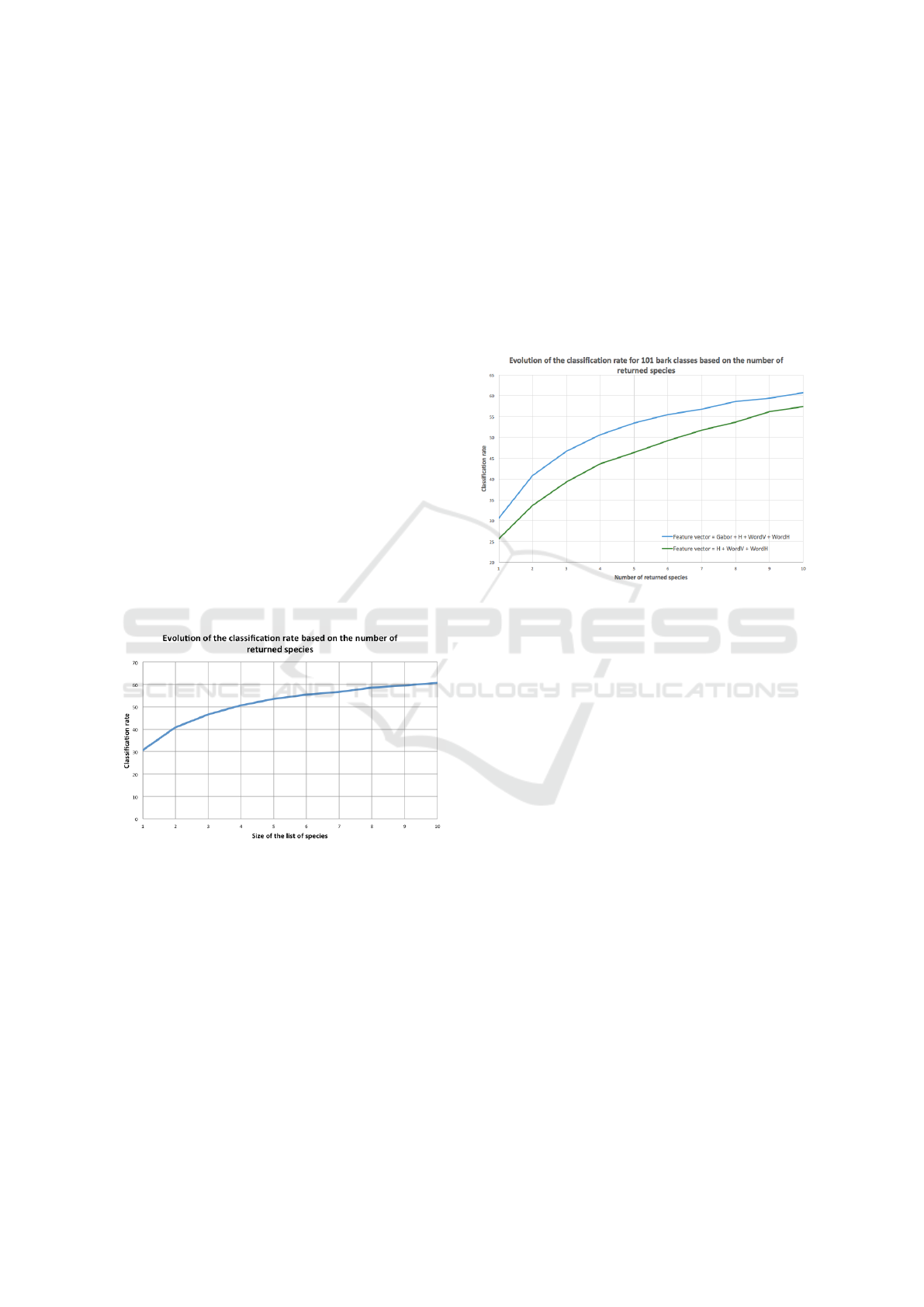
In the case of a smart-phone application, we can

propose to the user a list of tree species which most

likely match the tree he photographed. The Figure 8

shows the evolution of the classiﬁcation rate accord-

ing to the number of top answers returned. As said be-

fore, for a query bark image, we compute the probab-

ility of belonging to a species for each 1-vs-all binary

SVM. We order them in decreasing order the probab-

ility and check if the true species is in the top one, top

two, top three, and so on until top ten.

Figure 8: Evolution of the classiﬁcation rate.

Obviously the classiﬁcation rate increase with the

number of proposed species. It gains 10% when we

consider two species, and we have one chance out of

two to have the true species with a list of 4 proposi-

tions. Then progression of the recognition rate slow

down. Thus, at the end, the right species has a 60,8%

chance of being among the ﬁrst ten returned species.

3.2 Discussion Concerning the Inﬂuence

of Our Bark Features

We would like to give details of the choices of our

features vectors. First, to describe the structure of the

bark, we developed W

and W

, and add information

from bark image ﬁltered with Gabor. We can think

that the two ”vertical and horizontal words” already

capture the information given by Gabor. So we ana-

lyzed the classiﬁcation results when the feature vector

is composed of the two ”words”, the hue canal and

Gabor vector, and when it is composed of only the

two ”words” and the hue canal. Results are visible

on Figure 9, which represents the classiﬁcation rate

obtained if we return to the user a list of one, two or

more possible species.

Figure 9: Evolution of the classiﬁcation rate with and

without the features extracted through Gabor.

As we can see, the classiﬁcation rates when we

do not take into account the Gabor vector are inferior

compared to the ones obtained with the complete fea-

ture vector. Indeed, we lose on average 5% of right

classiﬁcation on the classiﬁcation rates depending on

the size of the list of returned species.

On the other hand, we studied the inﬂuence of the

frequency of the grid used to compute the ”vertical

word” W

and the ”horizontal word” W

. We com-

puted the classiﬁcation rate while varying the number

of columns and lines of the grid respectively corres-

ponding to W

and W

. We plan to give the user of

the smart-phone application a list of ﬁve possible spe-

cies. On Figure 10, we can see the evolution of the

classiﬁcation rate for the top 5 returned species.

Our results in section 3.1 are obtained with a grid

composed of 70 columns and 50 rows. We are limited

to 70 columns because the pixel widths of some of our

train bark images are too small. On Figure 10, we can

see that the best classiﬁcation rate is obtained when

the number of rows of the grid is 50 and the num-

ber of columns is 70. When the number of columns

is reduced, we can see that the classiﬁcation rate de-

creases. Finally, the ﬁner the grid is, the higher the

classiﬁcation rate is because the grid gets precise in-

formation.

Bark Recognition to Improve Leaf-based Classiﬁcation in Didactic Tree Species Identiﬁcation

439

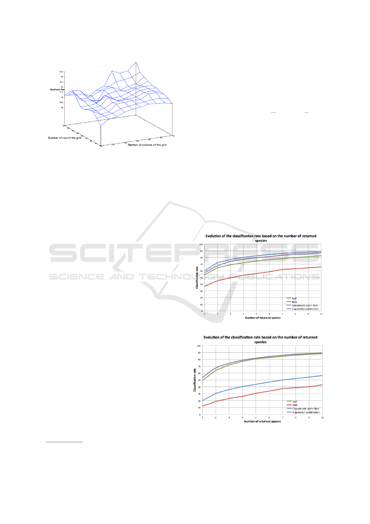
Figure 10: Inﬂuence of the frequency of the grid for the

computation of W

and W

3.3 Inﬂuence of Bark Processing in Tree

Leaves Classiﬁcation

Most of the time, the leaves and the bark of a tree can

be observable by a person who wants to know the spe-

cies of a tree. In order to take advantage of this double

source of information, we combine the recognition of

the bark with the recognition of the leaf previously

developed and integrated to Folia

, the leaf identiﬁca-

tion mobile application based on the work of (Cerutti

et al., 2013). We propose two combination methods.

First we concatenate the features of the leaf and the

features of the bark, and we use either the 1-vs-all

SVM classiﬁer or the classiﬁer used in the Folia ap-

plication (see (Cerutti et al., 2013)) for more inform-

ation). Secondly, we make an a posteriori combina-

tion, i.e. we do classiﬁcations independently for the

bark and for the leaf, then we combine the results of

the two classiﬁcations.

The Folia application uses a Gaussian nearest

neighbor classiﬁcation in which the classiﬁer builds a

model of each species S as a multi-dimensional Gaus-

sian distribution of its feature vectors, and estimates

the distance of a new sample represented by its fea-

ture vector F

to all the species models. To avoid that

the species with a high variability absorb less vari-

able classes, the distance d

GNN

, S) is computed as

the Euclidean distance to the surface of the hyper-

ellipsoid deﬁned by the centroid and covariance ma-

trix of the species. The result of this classiﬁcation is

the species that achieves the minimal distance. The

same classiﬁcation approach can be used for the bark

features F

and the concatenated feature vector F

b,l

Our a posteriori combination method uses all the

answers of the classiﬁers under the form of conﬁ-

dences (between 0 and 1) associated with each spe-

http://liris.univ-lyon2.fr/reves/folia

cies. The SVM classiﬁer already returns a conﬁ-

dences value c

SV M

(F, S) and a similar value can be

computed from the Folia classiﬁer: c

GNN

(F, S) =

−



GNN

(F,S)



. Then, the combination is performed

as a multiplicative fusion of the conﬁdence values for

each species:

⊗

c (F

, F

, S) =



c(F

, S)





c(F

, S)



(5)

with ω

and ω

the leaf and bark weighting (6)

The resulting conﬁdence

⊗

c is used to rank the spe-

cies and the classiﬁcation answer is the species cor-

responding to the highest combined conﬁdence.

We tested these two combination approaches on

a dataset of couples of bark and leaf images corres-

ponding the same species, for which we extracted re-

spectively the bark features presented in this article

and the leaf shape features from the folia application.

The leaf images are also from the Pl@ntView data-

base. However, some tree species have leaf image but

no bark image, and vice versa. Thereby, the number

of species we consider is reduced to 72.

Figure 11: Classiﬁcation with 1-vs-All SVM classiﬁer.

Figure 12: Classiﬁcation with k-nn classiﬁer from Folia.

On Figure 11 and Figure 12, we can see the evo-

lution of the classiﬁcation rate for the different me-

VISAPP 2017 - International Conference on Computer Vision Theory and Applications

440

thods. As we have reduced the number of classes, we

observe as expected an improvement in the bark clas-

siﬁcation rate (red curve on Figure 11). But we can

see that the classiﬁer used in the Folia application is

really not suitable for the bark feature vector (Figure

12). For the leaf classiﬁcation (green curve), the 1-

vs-all SVM classiﬁer improves the classiﬁcation rate

for the top 1 predicted species, but from the top 3 spe-

cies, the Folia classiﬁer gives better results. We can

note that when the two feature vectors (leaf+bark) are

concatenated (blue curves), the SVM classiﬁer (Fig-

ure 11) gives doubtlessly higher result than the Folia

classiﬁer (Figure 12). The classiﬁer used in Folia is in

fact not really suitable for longer vector.

Regarding the a posteriori combination (purple

curves), taking into account the bark improves the

classiﬁcation rate when the leaf and the bark are re-

cognized with the Folia classiﬁer (Figure 12). But the

performance are below the result with the concatenate

vector with SVM (Figure 11). With the classiﬁer used

for the bark (one-vs-all SVM, Figure 11), the a poste-

riori combination show an improvement in the tree re-

cognition when we take into account the bark and not

only the leaf (purple curve). Yet it gives slightly worse

results than when we supply the SVM with a conca-

tenated feature vector of leaf and bark (blue curve).

In conclusion, we reach the best classiﬁcation res-

ults when the features vectors of the bark and the leaf

are concatenated and classiﬁed with the 1-vs-all SVM

classiﬁer.

4 CONCLUSION

In this article, we proposed an original method for

the identiﬁcation of plant species to recognize trees

through the bark based on features used by botanists.

Our results achieve the same level as the state of the

art with a relatively short vector. We consider that

our method can be run with a limited computational

power and bearable by a smart-phone.

We also showed that taking into account the bark

can improve the recognition rate of trees obtained

only via the leaves. In a further work, we plan to im-

prove the combination of the bark classiﬁcation and

the leaf classiﬁcation by considering the results of the

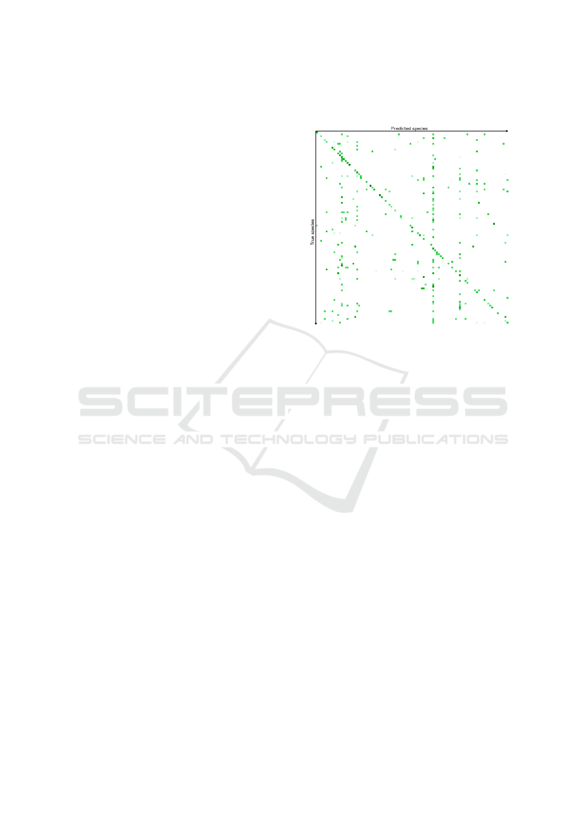
confusion matrix. As a matter of fact, if we take a

look to the confusion matrix of our bark classiﬁcation

on Figure 13, we can notice that some barks are more

predicted than they should. Indeed, we can clearly

see some columns where there are a lot of boxes are

green. It is the case for the classes where we have a

lot of samples and a lot of variability in the bark. In a

further work, we plan to take into account the results

in this matrix to moderate the belief in bark results

versus leaf results.

Figure 13: Confusion matrix: the greener the case, the

greater the occurrences.

Moreover, as we plan to create an educational

botanical smart-phone application, we would like to

translate the data from our features vectors as tan-

gible information for the user. For example, from the

hue histogram H, we would like to tell the user that

the bark of the tree is brown, gray, or yellowish, and

with G, W

and W

tell about the structure of the bark

(scales, strips, ridges, smooth, etc). Giving these in-

formation to the novice should help him to recognize

tree species on his own.

Furthermore, we developed W

and W

for tree

bark recognition, but we think that this concept could

be applied to other contexts where texture character-

ization is important.

Finally, in order to further improve the tree recog-

nition, we also want to extract features on the other

organs of the tree, such as the ﬂowers, which are the

reproductive organs of the plant and therefore charac-

teristic of the species, and also the fruits, which are

characteristic of the genus.

ACKNOWLEDGMENTS

This work is part of ReVeRIES project (Reconnais-

sance de Vegetaux Recreative, Interactive et Educat-

ive sur Smartphone) supported by the French Na-

tional Agency for Research with the reference ANR-

15-CE38-004-01.

Bark Recognition to Improve Leaf-based Classiﬁcation in Didactic Tree Species Identiﬁcation

441

REFERENCES

Bakic, V., Mouine, S., Ouertani-Litayem, S., Verroust-

Blondet, A., Yahiaoui, I., Go

eau, H., and Joly,

A. (2013). Inria’s participation at imageclef 2013

plant identiﬁcation task. In CLEF (Online Working

Notes/Labs/Workshop) 2013.

Bay, H., Tuytelaars, T., and Van Gool, L. (2006). Surf:

Speeded up robust features. In Computer vision–

ECCV 2006, pages 404–417. Springer.

Canny, J. (1986). A computational approach to edge detec-

tion. Pattern Analysis and Machine Intelligence, IEEE

Transactions on, (6):679–698.

Cerutti, G., Tougne, L., Mille, J., Vacavant, A., and Coquin,

D. (2013). Understanding leaves in natural images–

a model-based approach for tree species identiﬁca-

tion. Computer Vision and Image Understanding,

117(10):1482–1501.

eau, H., Bonnet, P., and Joly, A. (2015). Lifeclef plant

identiﬁcation task 2015. CEUR-WS.

eau, H., Bonnet, P., Joly, A., Baki

c, V., Barbe, J.,

Yahiaoui, I., Selmi, S., Carr

e, J., Barth

emy, D.,

Boujemaa, N., et al. (2013a). Pl@ntnet mobile app.

In Proceedings of the 21st ACM international confer-

ence on Multimedia, pages 423–424. ACM.

eau, H., Bonnet, P., Joly, A., Bakic, V., Barth

emy, D.,

Boujemaa, N., and Molino, J.-F. (2013b). The image-

clef 2013 plant identiﬁcation task. In CLEF.

eau, H., Bonnet, P., Joly, A., Boujemaa, N., Barth

emy,

D., Molino, J.-F., Birnbaum, P., Mouysset, E., and Pi-

card, M. (2011). The imageclef 2011 plant images

classi cation task. In ImageCLEF 2011, pages 0–0.

eau, H., Joly, A., Bonnet, P., Selmi, S., Molino, J.-F.,

Barth

emy, D., and Boujemaa, N. (2014). Lifeclef

plant identiﬁcation task 2014. In CLEF2014 Work-

ing Notes. Working Notes for CLEF 2014 Conference,

Shefﬁeld, UK, September 15-18, 2014, pages 598–

615. CEUR-WS.

Huang, Z.-K., Huang, D.-S., Du, J.-X., Quan, Z.-H., and

Guo, S.-B. (2006). Bark classiﬁcation based on gabor

ﬁlter features using rbpnn neural network. In Neural

Information Processing, pages 80–87. Springer.

Kumar, N., Belhumeur, P. N., Biswas, A., Jacobs, D. W.,

Kress, W. J., Lopez, I. C., and Soares, J. V. (2012).

Leafsnap: A computer vision system for automatic

plant species identiﬁcation. In Computer Vision–

ECCV 2012, pages 502–516. Springer.

Lowe, D. G. (1999). Object recognition from local scale-

invariant features. In Computer vision, 1999. The pro-

ceedings of the seventh IEEE international conference

on, volume 2, pages 1150–1157. Ieee.

Nakayama, H. (2013). Nlab-utokyo at imageclef 2013 plant

identiﬁcation task. In Working notes of CLEF 2013

conference.

Ojala, T., Pietik

ainen, M., and Harwood, D. (1996). A com-

parative study of texture measures with classiﬁcation

based on featured distributions. Pattern recognition,

29(1):51–59.

Szegedy, C., Liu, W., Jia, Y., Sermanet, P., Reed, S.,

Anguelov, D., Erhan, D., Vanhoucke, V., and Ra-

binovich, A. (2015). Going deeper with convolutions.

In Proceedings of the IEEE Conference on Computer

Vision and Pattern Recognition, pages 1–9.

Vapnik, V. N. (1999). An overview of statistical learn-

ing theory. Neural Networks, IEEE Transactions on,

10(5):988–999.

Wojtech, M. (2011). Bark: A Field Guide to Trees of the

Northeast. University Press of New England.

VISAPP 2017 - International Conference on Computer Vision Theory and Applications

442