LBP Histogram Selection based on Sparse Representation for Color
Texture Classification
Vinh Truong Hoang, Alice Porebski, Nicolas Vandenbroucke and Denis Hamad
Laboratoire d’Informatique Signal et Image de la Cˆote d’Opale,
50, rue Ferdinand Buisson, BP 719, 62228 Calais Cedex, France
Keywords:
Histogram Selection, Feature Selection, LBP Color Histogram, Texture Classification, Sparse Representation.
Abstract:
In computer vision fields, LBP histogram selection techniques are mainly applied to reduce the dimension
of color texture space in order to increase the classification performances. This paper proposes a new his-
togram selection score based on Jeffrey distance and sparse similarity matrix obtained by sparse representa-
tion. Experimental results on three benchmark texture databases show that the proposed method improves the
performance of color texture classification represented in different color spaces.
1 INTRODUCTION
Texture classification is a fundamental task in image
processing and computer vision. It is an important
step in many applications such as content-based im-
age retrieval, face recognition, object detection and
many more. Texture analysis methods was firstly de-
signed for dealing with gray-scale images. Among
the proposed approaches in the recent years to repre-
sent the texture images, Local Binary Pattern (LBP)
proposed by Ojala et al. has been known as one of the
most successful statistical approaches due to its effi-
cacy, robustness against illumination changes and rel-
ative fast calculation (Ojala et al., 1996; Ojala et al.,
2001; Pietik¨ainen et al., 2002; Ojala et al., 2002b). In
order to encode LBP, the gray level of each pixel is
compared with those of its neighbors and the results
of these comparisons are weighted and summed. The
obtained texture feature is the LBP histogram whose
bin count depends on the number of neighbors.
Otherwise, it has been demonstrated that color in-
formation is very important to represent the texture,
especially natural textures (Asada and Matsuyama,
1992). However, the extension of LBP to color leads
to consider several LBP histograms and only some of
which are relevant for texture classification. That is
the reason why many approaches have been proposed
to reduce the dimension of the feature space based on
the LBP histogram in order to improve the classifi-
cation performances (Zhang and Xu, 2015; Porebski
et al., 2013b; Guo et al., 2012; Zhou et al., 2013b;
Mehta and Egiazarian, 2016; Ren et al., 2015). The
dimensionality reduction consists to select the perti-
nent histogram bins. Another dimensional reduction
method was proposed by Porebski et al. which fo-
cus on selecting LBP histograms in their entirety. For
this purpose they introduce the Intra-Class Similar-
ity score (ICS-score) based on the similarity of the
textures within the different classes (Porebski et al.,
2013a). Kalakech et al. introduced another histogram
selection score, named ”Adapted Supervised Lapla-
cian score” (ASL-score) based on Jeffreydistance and
a similarity matrix (Kalakech et al., 2015). This ma-
trix is deduced from the class labels. It is a hard value
which is 0 or 1.
In this paper, we propose to extend the ASL-score
by using sparse representation to build a soft similar-
ity matrix that takes values between 0 and 1. Indeed,
in the past few years, sparse representation has been
successfully applied in signal and image processing
fields and provento be an effective tool for feature se-
lection (Qiao et al., 2010; Xu et al., 2013; Zhou et al.,
2013a). Moreover, the soft value of the similarity ob-
tained by the sparse representation could better reflect
the geometric structure of different classes. Indeed a
value between 0 and 1 will measure the similarity in
a subtle way, instead of being binary with just two
values 0 and 1. This may lead to more powerful dis-
criminating information. The proposed score, called
Sparse Adapted Supervised Laplacian score (SpASL-
score) will be evaluated thanks to several benchmark
color texture databases represented in different color
spaces.
In the following, we describe, in section 2, the
476
Hoang V., Porebski A., Vandenbroucke N. and Hamad D.
LBP Histogram Selection based on Sparse Representation for Color Texture Classification.
DOI: 10.5220/0006128204760483
In Proceedings of the 12th International Joint Conference on Computer Vision, Imaging and Computer Graphics Theory and Applications (VISIGRAPP 2017), pages 476-483
ISBN: 978-989-758-225-7
Copyright
c
 2017 by SCITEPRESS – Science and Technology Publications, Lda. All rights reserved

color LBP histograms. Section 3 presents the his-
togram selection approach and introduce the ASL-
score, while section 4, presents sparse representa-
tion for histogram selection and the proposed SpASL-
score. In section 5, experimental results indicate
that our score achieves better performances than pre-
vious works under several benchmark color texture
databases.
2 COLOR LBP HISTOGRAM
The LBP operator has been introduced by Ojala et al.
in 1996 to describe the textures present in gray-scale
images (Ojala et al., 1996). An extension to color im-
ages is proposed by M¨aenp¨a¨a et al. and used in sev-
eral color texture classification problems (M¨aenp¨a¨a
and Pietik¨ainen, 2004; Pietik¨ainen et al., 2011). The
color information of a pixel is characterized by three
color component in a 3-dimensional color space, de-
noted here C
1
C
2
C
3
. The color LBP operator con-
sists in assigning to each pixel a label which char-
acterizes the local pattern in a neighborhood. Each
label is a binary number calculated by thresholding
the color component of the neighbors by using the
color component of the considered pixel. The re-
sult of the thresholding, performed for each neigh-
bor pixel, is then coded by a weight mask. As do
Ojala et al. when they introduce the original LBP
operator, the 3 × 3 pixels neighborhood is consid-
ered. To characterize the local pattern of the consid-
ered pixel, the weighted values are finally summed
so that each label ranges from 0 to 255. In order to
characterize the whole color texture image, the LBP
operator is applied on each pixel and for each pair
of components. The corresponding distributions are
thus represented in nine different histograms: three
within-component LBP histograms ((C
1
,C
1
), (C
2
,C
2
)
and (C
3
,C
3
)) and six between-component LBP his-
tograms ((C
1
,C
2
), (C
2
,C
1
), (C
1
,C
3
), (C
3
,C
1
), (C
2
,C
3
)
and (C
3
,C
2
)). A color texture is thus represented in a
(9 × 256)-dimensional feature space. This results in
a high dimensional space, which could decrease the
classification performance. For this, it would be in-
teresting to find the most relevant histograms.
3 HISTOGRAM SELECTION
APPROACH
Histogram selection approaches are usually grouped
in three ways: filters, wrappers and embedded. The
latter combines the reduction of processing time of a
filter approach and the high performances of a wrap-
per approach. Filter approaches consist in computing
the score of each histogram in order to measure its ef-
ficiency. Then, the histograms are ranked according
to the proposed score. In wrapper approaches, his-
tograms are evaluated thanks to a specific classifier
and the selected ones are those which maximizes the
classification rate.
In the considered LBP histogram selection con-
text, the database is composed of N color texture im-
ages, each ones is characterized by 9 histograms. This
leads to 9 matrices H
r
, which are defined by:
H
r
=

h
r
1
...h
r
i
...h
r
N

=





h
r
1
(0) ... h
r
i
(0) ... h
r
N
(0)
... ... ... ... ...
h
r
1
(k) ... h
r
i
(k) ... h
r
N
(k)
... ... ... ... ...
h
r
1
(Q) ... h
r
i
(Q) ... h
r
N
(Q)





(1)
where, r = 1, 2, ..,9 and Q being the quantization
level.
Several measures have been proposed for evaluat-
ing difference between two histograms like Kullback-
Leibler, χ
2
, earth movers, Jeffrey, etc. (Cha and Sri-
hari, 2002). Jeffrey distance has the advantage of be-
ing positive and symmetric. It is defined by:
J(h
r
i
, h
r
j
) =
Q
∑
k=1
h
r
i
(k)log

h
r
i
(k)
h
r
i
(k)+h
r
j
(k)
2

+
Q
∑
k=1
h
r
j
(k)log

h
r
j
(k)
h
r
i
(k)+h
r
j
(k)
2

(2)
In (Kalakech et al., 2015), the Jeffrey distance is
used to construct an Adapted Laplacian score ASL
r
of
the r
th
histogram:
ASL
r
=
∑
N
i=1
∑
N
j=1
J(h
r
i
, h
r
j
)s
ij
∑
N
i=1
J(h
r
i
,
h
r
)d
i
(3)
h
r
is the histogram average:
h
r
=
∑
N
i=1
h
r
i
d
i
∑
N
i=1
d
i
(4)
where, d
i
is the local density of image I
i
defined by:
d
i
=
N
∑
j=1
s
ij
(5)
where, s
ij
is an element of the similarity matrix S. In
a supervised context, for each image I
i
, a class label
is associated y
i
. The similarity between two images I
i
and I
j
is defined by:
s
ij
=
(
1 if y
i
= y
j
,
0 otherwise
(6)
LBP Histogram Selection based on Sparse Representation for Color Texture Classification
477

In the next section, instead of using hard similarity
s
ij
labels, we will define the similarity matrix from
the sparse representation, and then integrate it into the
Equation (3).
4 SPARSE REPRESENTATION
FOR HISTOGRAM SELECTION
Recently, many works have been focused on sparse
linear representation to characterize data (Zhou et al.,
2013a; Xu et al., 2013; Zhu et al., 2013). The
sparse representation is based on the hypothesis that
each image is reconstructed through a linear combi-
nation of other images of the database. The modified
sparse representation based on l
1
-norm minimization
problem is used to construct the l
1
-graph adjacency
structure and a sparse similarity matrix automatically.
In (Qiao et al., 2010; Liu and Zhang, 2014) the sparse
representation is applied to feature selection in unsu-
pervised and supervised contexts. In this section, we
propose to use sparse similarity matrix combined with
Jeffrey distance for histogram selection in the super-
vised context.
4.1 Sparse Similarity Matrix
The modified sparse representation framework has
been proposed in order to construct a sparse similarity
matrix by finding the most compact representation of
data (Qiao et al., 2010). Given an image I
i
, character-
ized by histograms h
r
i
, r = 1, 2,..9, and a histogram
matrix H
r
of Equation 1 contains the elements of an
over-complete dictionary in its columns. The goal of
sparse representation of h
r
i
is to estimate by using a
few entries of H
r
as possible.
min
s
i
ks
i
k
1
, s.t. h
r
i
= H
r
s
i
, 1 = 1
T
s
i
, (7)
where s
i
∈ ℜ
N
is the coefficient vector. It is defined
as:
s
i
= [s
i,1
, ..., s
i,i−1
, 0, s
i,i+1
, ..., s
i,N
]
T
(8)
s
i
is an N-dimensional vector in which the i
th
element
is equal to zero implying that h
r
i
is removed from H
r
.
ks
i
k
1
is the l
1
-norm of s
i
and 1 ∈ ℜ
N
is a vector of all
ones.
For each sample h
r
i
, we can compute the similarity
vector
ˆ
s
i
, and then get the sparse similarity matrix:
S = [
ˆ
s
1
,
ˆ
s
2
, ...,
ˆ
s
N
]
T
, (9)
where
ˆ
s
i
is the optimal solution of Equation (7). The
matrix S determines both graph adjacency structure
and sparse similarity matrix simultaneously. Note
that, the sparse similarity matrix is generally asym-
metric.
Since the real-world images contain noise, the fol-
lowing objective function is used:
min
s
i
ks
i
k
1
, s.t. kh
r
i
− H
r
s
i
k
2
< δ, 1 = 1
T
s
i
,
(10)
where, δ represents the error tolerance which is cho-
sen to 10
−4
in our experiments. k.k
2
denotes l
2
-norm
of a vector. This problem can be solved in a poly-
nomial time with standard linear programming meth-
ods (Qiao et al., 2010).
4.2 Sparse Adapted Superived
Laplacian Score
In this section, the sparse similarity matrix defined by
sparse representation is applied in the supervised con-
text. Given a database of N images belonging to P
classes, each class p, p = 1, .., P, contains N
p
images.
For each class, we construct the sparse similarity ma-
trix using images within the same class by Equation
(10). We note S
p
the sparse similarity matrix of class
p, and h
rp
i
the r
th
histogram of image I
i
in class p.
We notice that the similarity in Equation (6) is hard, it
takes the value 1 if the two corresponding images are
in the same class and the value 0 if theyare in different
classes. On the other side, the sparse reconstruction
in Equation (10) allows us to determine the soft sim-
ilarity value between 0 and 1 for two corresponding
images. This soft value could then reflect the intrin-
sic geometric properties of classes which may lead to
natural discriminating information.
Integrating the sparse similarity matrix into Equa-
tion (3) leads to Sparse Adapted Supervised Laplacian
score (SpASL) defined by:
SpASL
r
=
∑
P
p=1
∑
N
p
i, j=1
J(h
rp
i
, h
rp
j
) ˆs
p
ij
∑
P
p=1
∑
N
p
i=1
J(h
rp
i
,
h
rp
)d
p
i
(11)
where, r = 1, 2, ...9 is the histogram index, N
p
is the
number of images of the p
th
class, ˆs
p
ij
is the element
of the sparse matrix S
p
related to the p
th
class. His-
togram selection consists to compute for each of all
9 histograms the associated SpASL-score and to rank
histograms according to their scores in ascending or-
der.
5 EXPERIMENTAL RESULTS
In order to evaluate the efficiency of the proposed
score, we perform the evaluation on three bench-
VISAPP 2017 - International Conference on Computer Vision Theory and Applications
478

9 LBP Histograms
… …
Histogram
Selec on
✁
✁
✁
Image
Color space
C
C
C
AC
Classificaon
LBP
1
2
3
Figure 1: LBP histogram selection scheme.
marks color texture images databases: Outex-TC-
0003
1
, New BarkTex and USPTex
2
Note that, each color texture is characterized by
9 LBP histograms. Color texture can be repre-
sented in different color spaces, which can be grouped
in four families: the primary color spaces, the lu-
minance–chrominance color spaces, the perceptual
spaces and the independent axis color spaces (Qazi
et al., 2011). In our experiments, we used the follow-
ing color spaces: RGB, HSV, HLS, ISH, rgb, b
w
r
g
b
y
,
I-HLS, I
1
I
2
I
3
, YC
b
C
r
, YIQ, Luv, Lab, XYZ, YUV.
Figure 1 shows the LBP histogram selection scheme
in one color space. In the experiments, we com-
pare our SpASL-score for histogram selection with
the original ASL-score proposed in (Kalakech et al.,
2015) and the ICS-score proposed in (Porebski et al.,
2013b). Each database is divided into training set
and testing set, as shown in Table 1. The training
set is used for histogram ranking procedure by apply-
ing Equation (11). Then, ranked histograms are used
as inputs to classification process which is performed
based on testing set. The L1-distance is associated
with 1-NN classifier while the classification perfor-
mance is evaluated by accuracy rate (AC). For every
subsection below, we present a short description of
the image databases and analyze the obtained experi-
mental results.
5.1 Experiments on BarkTex Database
BarkTex database includes six tree bark classes ac-
quired under natural (daylight) illumination condi-
tions (Lakmann, 1998). The version New Barktex
has been built by Porebski et al. (Porebski et al.,
2014). Table 2 presents the results on New Bark-
tex database. For each color space, the accuracy rate
applied on testing images and the number of the se-
lected LBP histogram reached (in parentheses) are
computed. The first rows shows the results obtained
by ICS, ASL, SpASL-score and without selection in
1
The Outex-TC-0003 image test suite can be down-
loaded at http://www.cse.oulu.fi/CMV
2
The BarkTex and USPTex image test suites can be
downloaded at
https://www.lisic.univ-littoral.fr/
˜ porebski/Recherche.html
RGB color space. They give exactly the same AC
(81.25) with 4 histograms selected. By examining the
selected histogram in this color space, we notice that
all 3 scores used three within-component LBP his-
tograms (RR, GG, BB) and one between-component
LBP histogram (RG). The last row of Table 2 shows
the mean AC of 14 color spaces used. We can see that
the performance of SpASL-score is slightly higher or
equal than ASL-score. The average AC of SpASL-
score is better than ICS and ASL-score. The best
results obtained is 81.37 by ICS-score in YIQ space
while ASL and SpASL give the same results. The
maximal number of histograms selected is 9 for Luv
space while the minimal is 2 for XYZ and I-HLS
spaces. It is interesting to note that, ASL and SpASL
give within-component LBP histograms as the best
score globally while ICS assigns the best score differ-
ently. This result can show the effectiveness of sparse
similarity matrix given by the proposed score.
5.2 Experiments on Outex-TC-00013
Database
The test suite Outex-TC-00013 is provided by the
Outex texture database (Ojala et al., 2002a). This
database composes collection of natural materials ac-
quired under three-CCD color camera under the same
controlled conditions. Table 3 presents the results on
Outex-TC-00013 database.
In most of cases, SpASL gives better results than
ASL and ICS, except in I
1
I
2
I
3
color space. The aver-
age AC of SpASL-score is better than ICS and ASL-
score. The best result (93.38) is reached by RGB and
HLS with 8 histogram selected. The minimal number
of histogram selected is 6 for rgb and YC
b
C
r
spaces.
As the same for BarkTex database, we notice that
SpASL and ASL give within-component LBP his-
tograms as the best score over most of color spaces,
except in Luv space.
5.3 Experiments on USPTex Database
The USPTex database has textures typically found in
daily life, such as beans, rice, tissues, road scenes,
LBP Histogram Selection based on Sparse Representation for Color Texture Classification
479

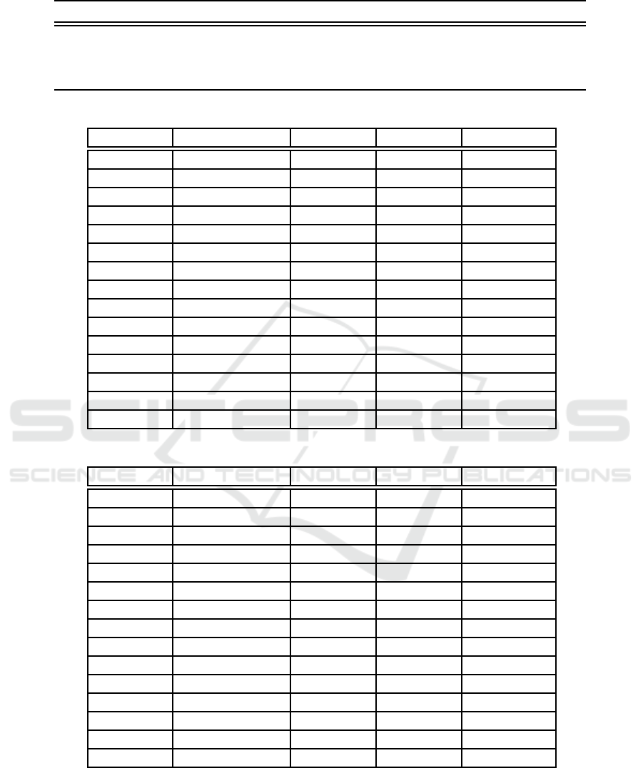
Table 1: Summary of image databases used in experiment.
Dataset name Image size # class # training # test Total
New BarkTex (Porebski et al., 2014) 64 × 64 6 816 816 1632
Outex-TC-00013 (Ojala et al., 2002a) 128 × 128 68 680 680 1360
USPTex (Backes et al., 2012) 128 × 128 191 1146 1146 2292
Table 2: Experiments on BarkTex database.
Color space Without selection ICS-score ASL-score SpASL-score
RGB 73.28 (9) 81.25 (4) 81.25 (4) 81.25 (4)
rgb 74.39 (9) 76.84 (7) 77.08 (3) 77.08 (3)
I
1
I
2
I
3
71.69 (9) 79.53 (7) 79.53 (7) 79.53 (7)
HSV 70.47 (9) 81.00 (3) 81.00 (3) 81.00 (3)
b
w
r
g
b
y
72.06 (9) 80.02 (7) 80.64 (6) 80.64 (6)
HLS 70.10 (9) 81.00 (3) 81.00 (3) 81.00 (3)
I-HLS 72.06 (9) 75.86 (6) 77.08 (5) 78.80 (2)
ISH 71.69 (9) 79.78 (3) 79.78 (3) 79.78 (3)
YC
b
C
r
71.57 (9) 79.29 (7) 79.29 (7) 79.29 (7)
Luv 71.08 (9) 71.08 (9) 71.08 (9) 71.08 (9)
Lab 67.16 (9) 67.65 (7) 68.14 (6) 68.14 (6)
XYZ 76.10 (9) 78.19 (3) 78.19 (3) 78.68 (2)
YUV 71.81 (9) 78.92 (7) 78.92 (7) 78.92 (7)
YIQ 77.08 (9) 81.37 (6) 80.76 (7) 80.76 (7)
Average 72.18±2.48 77.98±4.04 78.12±3.90 78.28±3.89
Table 3: Experiments on Outex-TC-0003 database.
Color space Without selection ICS-score ASL-score SpASL-score
RGB 92.94 (9) 92.94 (9) 93.24 (8) 93.38 (8)
rgb 87.06 (9) 87.06 (9) 87.35 (8) 87.35 (6)
I
1
I
2
I
3
88.53 (9) 88.97 (8) 88.68 (6) 88.53 (9)
HSV 90.44 (9) 91.03 (8) 91.32 (7) 91.32 (7)
b
w
r
g
b
y
89.95 (9) 89.85 (9) 91.76 (8) 91.76 (8)
HLS 92.35 (9) 92.35 (9) 93.38 (6) 93.38 (6)
I-HLS 89.71 (9) 89.71 (9) 89.71 (9) 90.29 (7)
ISH 92.94 (9) 92.94 (9) 93.09 (8) 93.09 (8)
YC
b
C
r
89.56 (9) 89.56 (9) 90.59 (8) 90.59 (6)
Luv 90.29 (9) 90.29 (9) 90.29 (8) 90.29 (8)
Lab 89.56 (9) 90.00 (8) 89.85 (6) 89.85 (6)
XYZ 92.06 (9) 92.06 (9) 92.06 (9) 92.06 (9)
YIQ 88.82 (9) 88.82 (9) 88.97 (8) 89.26 (8)
YUV 89.56 (9) 89.56 (9) 90.44 (8) 90.44 (8)
Average 90.26±1.73 90.36±1.70 90.76±1.81 90.82±1.80
... (Backes et al., 2012). The natural color tex-
tures images are taken under an unknown but fixed
light source. Table 4 presents the results on USP-
Tex database. We can see that, SpASL outperforms
the ICS-score and slightly better than ASL-score for
all color spaces. The best AC obtained is 93.19 in
YUV space with only 3 histogram selected. Note that
ASL and SpASL-score give within-component LBP
histograms as the best score in all color spaces. The
results on USPTex confirm again the strength of the
VISAPP 2017 - International Conference on Computer Vision Theory and Applications
480

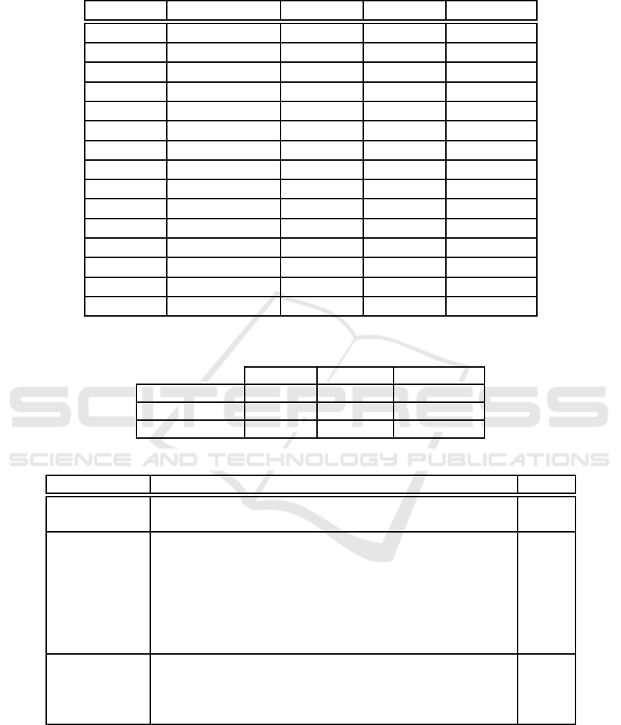
Table 4: Experiments on USPTex database.
Color space Without selection ICS-score ASL-score SpASL-score
RGB 89.53 (9) 90.31 (6) 91.27 (4) 91.27 (4)
rgb 78.36 (9) 83.25 (3) 83.25 (3) 83.25 (3)
I
1
I
2
I
3
75.39 (9) 82.46 (4) 92.06 (3) 92.06 (3)
HSV 83.25 (9) 85.78 (7) 90.40 (3) 90.40 (3)
b
w
r
g
b
y
77.23 (9) 86.21 (4) 92.41 (3) 92.41 (3)
HLS 81.59 (9) 85.08 (7) 90.31 (3) 90.31 (3)
I-HLS 83.42 (9) 87.00 (7) 91.27 (3) 91.27 (3)
ISH 82.90 (9) 86.04 (7) 90.40 (3) 90.40 (3)
YC
b
C
r
76.79 (9) 86.74 (4) 93.11 (3) 93.11 (3)
Luv 88.74 (9) 88.74 (9) 88.74 (9) 90.31 (3)
Lab 79.58 (9) 85.78 (7) 85.78 (7) 87.87 (3)
XYZ 89.79 (9) 90.84 (5) 90.92 (6) 91.01 (6)
YIQ 76.70 (9) 84.47 (4) 92.58 (3) 92.58 (3)
YUV 76.79 (9) 86.04 (4) 93.19 (3) 93.19 (3)
Average 81.43.26±5.04 86.38±2.36 90.40±2.82 90.67±2.55
Table 5: Classification performance under BarkTex, Outex-TC-00013 and USPTex image databases by histogram selection
approaches.
ICS-score ASL-score SpASL-score
BarkTex 81.37 (6) 81.25 (4) 81.25 (4)
OuTex-TC-0003 92.94 (9) 93.38 (8) 93.38 (8)
USPTex 90.84 (5) 93.19 (3) 93.19 (3)
Table 6: Classification performance under BarkTex, Outex-TC-00013 and USPTex image databases in the previous works.
Database Method Results
BarkTex
Compact descriptors color LBP (Ledoux et al., 2016) 79.40
MCSFS (Porebski et al., 2013b) 75.90
Outex-TC-0003
MCSFS (Porebski et al., 2013b) 96.60
Color histograms (M¨aenp¨a¨a and Pietik¨ainen, 2004) 95.40
Parametric spectral analysis (Qazi et al., 2011) 94.50
Compact descriptors color LBP (Ledoux et al., 2016) 92.50
Stat multi-model geodesic distance (El Maliani et al., 2014) 89.70
Block truncation coding (Guo et al., 2016) 88.24
Colour contrast occurrence matrix (Mart´ınez et al., 2015) 87.79
USPTex
Local jet space (Oliveira et al., 2015) 94.29
Block truncation coding (Guo et al., 2016) 93.94
Compact descriptors color LBP (Ledoux et al., 2016) 91.90
Fractal descriptors over the wavelet (Florindo and Bruno, 2016) 85.56
sparse similarity matrix integrated into the proposed
score which allows to improve the classification per-
formances.
5.4 Comparison with Previous Existing
Methods
Table 6 reports the classification performance with
different existing methods in literature under three
benchmark image databases. The Multi Color Space
LBP Histogram Selection based on Sparse Representation for Color Texture Classification
481

Feature Selection (MCSFS) is used for characterized
texture images with 28 color spaces in (Porebski et al.,
2013b). The results obtained are 75.90 on BarkTex
and 96.60 on OuTex-TC-0003. In (Ledoux et al.,
2016), the results obtained are 79.40 on BarkTex,
92.50 on OuTex-TC-0003 and 91.90 on USPTex by
using the compact color orders of LBP approach in
RGB space. By using local jet space, the best results
obtained on USPTex is 94.29 in (Oliveiraet al., 2015).
In order to compare those results, we summarize the
best classification performance by histogram selec-
tion approaches as shown in Table 5. As we can see,
the results obtained by histogram selection is promis-
ing by using different single color space.
6 CONCLUSION
Local Binary Pattern (LBP) is one of the most suc-
cessful approaches to characterize texture images. Its
extension to color information is very important to
represent natural texture images. However, color LBP
leads to consider several histograms, only some of
which are pertinent for texture classification. We
proposed a histogram selection score based on Jef-
frey distance and sparse similarity matrix obtained
by sparse representation. Experimental results are
achieved with OuTex-TC-00013, BarkTex and USP-
Tex databases. The proposed histogram selection
score, integrating soft similarities, improves the re-
sults of color texture classification. The works pre-
sented in this paper are now continued in order to ex-
tend in multi-color space and with different selection
strategies.
REFERENCES
Asada, N. and Matsuyama, T. (1992). Color image analy-
sis by varying camera aperture. In Pattern Recogni-
tion, 1992. Vol.I. Conference A: Computer Vision and
Applications, Proceedings., 11th IAPR International
Conference on, pages 466–469.
Backes, A. R., Casanova, D., and Bruno, O. M. (2012).
Color texture analysis based on fractal descriptors.
Pattern Recognition, 45(5):1984–1992.
Cha, S.-H. and Srihari, S. N. (2002). On measuring the
distance between histograms. Pattern Recognition,
35(6):1355–1370.
El Maliani, A. D., El Hassouni, M., Berthoumieu, Y.,
and Aboutajdine, D. (2014). Color texture classifi-
cation method based on a statistical multi-model and
geodesic distance. Journal of Visual Communication
and Image Representation, 25(7):1717–1725.
Florindo, J. and Bruno, O. (2016). Texture analysis by frac-
tal descriptors over the wavelet domain using a best
basis decomposition. Physica A: Statistical Mechan-
ics and its Applications, 444:415–427.
Guo, J.-M., Prasetyo, H., Lee, H., and Yao, C.-C. (2016).
Image retrieval using indexed histogram of Void-and-
Cluster Block Truncation Coding. Signal Processing,
123:143–156.
Guo, Y., Zhao, G., and Pietik¨ainen, M. (2012). Discrimina-
tive features for texture description. Pattern Recogni-
tion, 45(10):3834–3843.
Kalakech, M., Porebski, A., Vandenbroucke, N., and
Hamad, D. (2015). A new LBP histogram selection
score for color texture classification. In Image Pro-
cessing Theory, Tools and Applications (IPTA), 2015
International Conference on, pages 242–247.
Lakmann, R. (1998). Barktex benchmark database of color
textured images.
Ledoux, A., Losson, O., and Macaire, L. (2016). Color
local binary patterns: compact descriptors for tex-
ture classification. Journal of Electronic Imaging,
25(6):061404.
Liu, M. and Zhang, D. (2014). Sparsity score: a novel
graph-preserving feature selection method. Interna-
tional Journal of Pattern Recognition and Artificial
Intelligence, 28(04):1450009.
Mart´ınez, R. A., Richard, N., and Fernandez, C. (2015). Al-
ternative to colour feature classification using colour
contrast ocurrence matrix. In The International Con-
ference on Quality Control by Artificial Vision 2015,
pages 953405–953405. International Society for Op-
tics and Photonics.
Mehta, R. and Egiazarian, K. (2016). Dominant Rotated
Local Binary Patterns (DRLBP) for texture classifica-
tion. Pattern Recognition Letters, 71:16–22.
M¨aenp¨a¨a, T. and Pietik¨ainen, M. (2004). Classification
with color and texture: jointly or separately? Pattern
Recognition, 37(8):1629–1640.
Ojala, T., Maenpaa, T., Pietikainen, M., Viertola, J., Kyllo-
nen, J., and Huovinen, S. (2002a). Outex - new frame-
work for empirical evaluation of texture analysis algo-
rithms. In Pattern Recognition, 2002. Proceedings.
16th International Conference on, volume 1, pages
701–706 vol.1.
Ojala, T., Pietik¨ainen, M., and Harwood, D. (1996). A com-
parative study of texture measures with classification
based on featured distributions. Pattern Recognition,
29(1):51 – 59.
Ojala, T., Pietik¨ainen, M., and M¨aenp¨a¨a, T. (2001). A
Generalized Local Binary Pattern Operator for Mul-
tiresolution Gray Scale and Rotation Invariant Texture
Classification. In Proceedings of the Second Interna-
tional Conference on Advances in Pattern Recogni-
tion, ICAPR ’01, pages 397–406, London, UK, UK.
Springer-Verlag.
Ojala, T., Pietik¨ainen, M., and M¨aenp¨a¨a, T. (2002b). Mul-
tiresolution Gray-Scale and Rotation Invariant Tex-
ture Classification with Local Binary Patterns. IEEE
Trans. Pattern Anal. Mach. Intell., 24(7):971–987.
Oliveira, M. W. d. S., da Silva, N. R., Manzanera, A., and
Bruno, O. M. (2015). Feature extraction on local jet
space for texture classification. Physica A: Statistical
Mechanics and its Applications, 439:160–170.
VISAPP 2017 - International Conference on Computer Vision Theory and Applications
482

Pietik¨ainen, M., Hadid, A., Zhao, G., and Ahonen, T.
(2011). Computer Vision Using Local Binary Pat-
terns, volume 40. Springer London, London.
Pietik¨ainen, M., M¨aenp¨a¨a, T., and Viertola, J. (2002). Color
texture classification with color histograms and local
binary patterns. In Workshop on Texture Analysis in
Machine Vision, pages 109–112.
Porebski, A., Vandenbroucke, N., and Hamad, D. (2013a).
LBP histogram selection for supervised color texture
classification. In ICIP, pages 3239–3243.
Porebski, A., Vandenbroucke, N., and Macaire, L. (2013b).
Supervised texture classification: color space or tex-
ture feature selection? Pattern Analysis and Applica-
tions, 16(1):1–18.
Porebski, A., Vandenbroucke, N., Macaire, L., and Hamad,
D. (2014). A new benchmark image test suite for eval-
uating colour texture classification schemes. Multime-
dia Tools and Applications, 70(1):543–556.
Qazi, I.-U.-H., Alata, O., Burie, J.-C., Moussa, A., and
Fernandez-Maloigne, C. (2011). Choice of a perti-
nent color space for color texture characterization us-
ing parametric spectral analysis. Pattern Recognition,
44(1):16–31.
Qiao, L., Chen, S., and Tan, X. (2010). Sparsity preserv-
ing projections with applications to face recognition.
Pattern Recognition, 43(1):331–341.
Ren, J., Jiang, X., and Yuan, J. (2015). Learning LBP struc-
ture by maximizing the conditional mutual informa-
tion. Pattern Recognition, 48(10):3180–3190.
Xu, J., Yang, G., Man, H., and He, H. (2013). L1 graph
based on sparse coding for feature selection. In Ad-
vances in Neural Networks–ISNN 2013, pages 594–
601. Springer.
Zhang, Q. and Xu, Y. (2015). Block-based selection
random forest for texture classification using multi-
fractal spectrum feature. Neural Computing and Ap-
plications.
Zhou, G., Lu, Z., and Peng, Y. (2013a). L1-graph con-
struction using structured sparsity. Neurocomputing,
120(0):441 – 452.
Zhou, S.-R., Yin, J.-P., and Zhang, J.-M. (2013b). Lo-
cal binary pattern (LBP) and local phase quantization
(LBQ) based on Gabor filter for face representation.
Neurocomputing, 116:260–264.
Zhu, X., Wu, X., Ding, W., and Zhang, S. (2013). Feature
selection by joint graph sparse coding. In SDM, pages
803–811. SIAM.
LBP Histogram Selection based on Sparse Representation for Color Texture Classification
483