Localization and Mapping of Cheap Educational Robot with Low
Bandwidth Noisy IR Sensors
Muhammad Habib Mahmood
1,2
and Pere Ridao Rodriquez
2
1
Department of Electrical Engineering, Air University, Islamabad, Pakistan
2
Computer Vision and Robotics (ViCOROB) Institute, University of Girona, Girona, Spain
Keywords:
Localization, Mapping, Kalman Filter, Particle Filter, Occupancy Grid Mapping, Monte-Carlo Localization.
Abstract:
The advancements in robotics has given rise to the manufacturing of affordable educational mobile robots.
Due to their size and cost, they possess limited global localization and mapping capability. The purpose of
producing these robots is not fully materialized if advance algorithms cannot be demonstrated on them. In this
paper, we address this limitation by just using dead-reckoning and low bandwidth noisy infrared sensors for
localization in an unknown environment. We demonstrate Extended Kalman Filter implementation, produce
a map of the unknown environment by Occupancy grid mapping and based on this map, perform particle
filtering to do Monte-Carlo Localization. In our implementation, we use the low cost e-puck mobile robot,
which performs these tasks. We also putforth an empirical evaluation of the results, which shows convergence.
The presented results provide a base to further build on the navigation and path-planning problems.
1 INTRODUCTION
Localization in robotics is considered an old problem.
Many methods have been explored to formulate a so-
lution to this problem but as it is dependent on the
surrounding environment, all the solutions differ un-
der varying environmental conditions. Moreover, be-
sides the method, the result of localization is also de-
pendent on the sensors. While, the use of expensive
sensors with sophisticated hardware is necessary for
industrial use, the approach changes completely, if the
purpose is to use the robots for educational purposes.
Recently, researchers have shown particular in-
terest in low cost educational robots. Recent
works (S. Wang and Magnenat, 2016; S. Bazeille
and Filliat, 2015) show that their has been a growing
trend of trying to accommodate accessible low budget
robots in the academic environment. This approach
has been tried for mapping and navigation (S. Bazeille
and Filliat, 2015), multi-robot systems (J. McLurkin
and Bilstein, 2013), collaborative robots (A. Prorok
and Martinoli, 2012) etc. This trend finds its roots
from the idea that complex algorithms can be imple-
mented in low budget machines.
The robots used in education are build to be in-
expensive, containing low cost sensors with repeat-
able motor drives. The sensors mounted on these ma-
chines are highly susceptible to environmental noise.
The purpose of these robots is to visually demonstrate
theoretical concepts. If these robots are used in envi-
ronments where the effect of ambient sources adds to
the noise in sensing, then their repeatable utilization
suffers. On top of it, if advance robotics’ concepts are
tried to be tested, the robots tend to fail.
In this paper, we approach the problem of ro-
bustly implementing complex localization and map-
ping algorithms on an inexpensive e-puck robot with
low bandwidth infrared (IR) sensors in a probabilistic
framework. Utilizing dead-reckoning and overhead
camera, we perform Extended Kalman-Filter Local-
ization. Then, by using the low bandwidth IR noisy
sensor, we devise a map of an unknown environment
by the Occupancy Grid Mapping algorithm. The ac-
quired map is then utilized in the implementation of
particle filtering by Monte-Carlo Localization. A de-
tailed evaluation of the quantitative results of these
algorithms with convergence are also shown. It can
also be seen that the error in localization for all im-
plementations remains with in 3σ bound at all times.
2 RELATED WORK
The advent of robotics has given rise to several off-
shoots. Among these, recent trends by researchers
Mahmood, M. and Rodriguez, P.
Localization and Mapping of Cheap Educational Robot with Low Bandwidth Noisy IR Sensors.
DOI: 10.5220/0006204305830590
In Proceedings of the 6th International Conference on Pattern Recognition Applications and Methods (ICPRAM 2017), pages 583-590
ISBN: 978-989-758-222-6
Copyright
c
 2017 by SCITEPRESS – Science and Technology Publications, Lda. All rights reserved
583

suggests that there has been a growing interest in
using educational robots to implement and demon-
strate complex robotics algorithms. In an imple-
mentation, a mapping robot using RP Lidar scanner
was used (M. Markom and Shakaff, 2015). Though,
the implementation is for an indoor robot, the Lidar
sensor size makes its usage difficult in small sized
educational robots. Motion and pose tracking for
mobile robots was also proposed using open-source
off-the-shelf hardware and software (A.D. Cucci and
Matteucci, 2016), along with an experimental bench-
mark protocol for indoor navigation (C. Sprunk and
Jalobeanu, 2016). These implementations demand
high computational overheads, which might again be
difficult to sustain in a small educational robot.
On a different note, a localization approach us-
ing fixed remote surveillance cameras was also pro-
posed (Shim and Cho, 2016). However, this imple-
mentation can only be tested on a high cost design.
Another localization and mapping implementation,
with unknown noise characteristics, presented an ap-
plication of Simultaneous Localization and Mapping
(SLAM) (Ahmad and Namerikawa, 2010). This im-
plementation was also computationally extensive, un-
suitable for educational robots.
Several dedicated educational robots have also
been presented. e-puck was presented as a multi-
sensor table-top small mobile robot (F. Mondada
and Martinoli, 2009). Another one was Roomba,
which was a uniquitous mobile robot platform (Tri-
belhorn and Dodds, 2007). Similar frameworks for
low cost robot implementations with different ap-
proaches were presented as collaborative localiza-
tion (A. Prorok and Martinoli, 2012), multi-robot sys-
tem (J. McLurkin and Bilstein, 2013), mapping and
navigation (S. Bazeille and Filliat, 2015) and local-
ization (S. Wang and Magnenat, 2016).
A repeatable implementation of these advance al-
gorithms in low cost robots is a limitation, which per-
sists in these implementations. To overcome this, we
propose the implementation of EKF, OGM and MCL
in e-puck mobile robot. In the remaining sections,
section 3 explains the localization and mapping prob-
lem, section 4 describes the Experimental setup and
results, followed by a discussion in section 5 and con-
clusion in section 6.
3 LOCALIZATION AND
MAPPING
The localization and mapping algorithms were imple-
mented in the e-puck mobile robot. Initially, the local-
ization problem was addressed by Extended Kalman
Filter Localization (EKF Localization). Then, by us-
ing the noisy IR sensors, Occupancy Grid Mapping
of the unknown arena was performed. Finally, the
map was used in a particle filter framework to per-
form Monte-Carlo Localization.
3.1 EKF Localization
Extended Kalman Filter is an implementation of
Bayes Filter, which allows formulating the localiza-
tion problem as a Bayesian estimation problem. The
Bayes filter is derived from the Bayes Theorem and
it relates the conditional probabilities and the prior
probabilities of two events. EKF Localization algo-
rithm presented in (S. Thrun and Fox, 2005) is an ex-
tension of the Kalman Filter (KF). KF’s assumption of
linearity is rarely fulfilled in practice and EKF over-
comes this assumption of linearity by considering that
state transition probability and/or the measurement
probability can be non linear functions. The poste-
rior for true belief was estimated by approximating
a Gaussian, which was calculated using linearization
approximation. This got rid of transformation matri-
ces A
k
and B
k
and resulted in Jacobians G
k
and H
k
as
described in (S. Thrun and Fox, 2005).
Algorithm 1: EKF Localization.
1: procedure EKF( ˆx
k−1
,P
k−1
,u
k
,z
k
)
2: ˆx
−
k
= f ( ˆx
k−1
,u
k
,0)
3: P
−
k
= A
k
P
k−1
A
T
k
+W
k
Q
k
W
T
k
4: K
k
= P
−
k
H
T
k
(H
k
P
−
k
H
T
k
+V
k
R
k
V
T
k
)
−1
5: ˆx
−
k
+ K
k
(z
k
− h(ˆx
−
k
,0))
6: P
k
= (I − K
k
H
k
)P
−
k
7: return (x
k
,P
k
)
In Figure 1, the robot moved from Pose 1 in frame
{R − 1} to Pose 2 in frame {R}. The robot moved by
the vector x
k
k−1
given in robot frame {R − 1}. This
vector had to be compounded with x
B
k−1
to get x
B
k
.
The compounding function was a non linear func-
tion, which also had noise affect in it. This effect
was catered for by the inclusion of w
k
, which was
the noise associated with odometry (dead-reckoning),
having zero mean and a covariance matrix Q
k
. As the
cross covariance of the state variable was zero, the Q
k
matrix became a diagonal matrix. In the measurement
step, the robot pose with respect to the global frame
was estimated with the help of an overhead camera z
k
.
The update step was performed by using the mean
and covariance generated in the prediction step in
conjunction with the measurement z
k
and its noise v
k
.
In the update step, first the Kalman Gain K
k
was cal-
culated, using the value of V
k
. Then, the innovation
ICPRAM 2017 - 6th International Conference on Pattern Recognition Applications and Methods
584

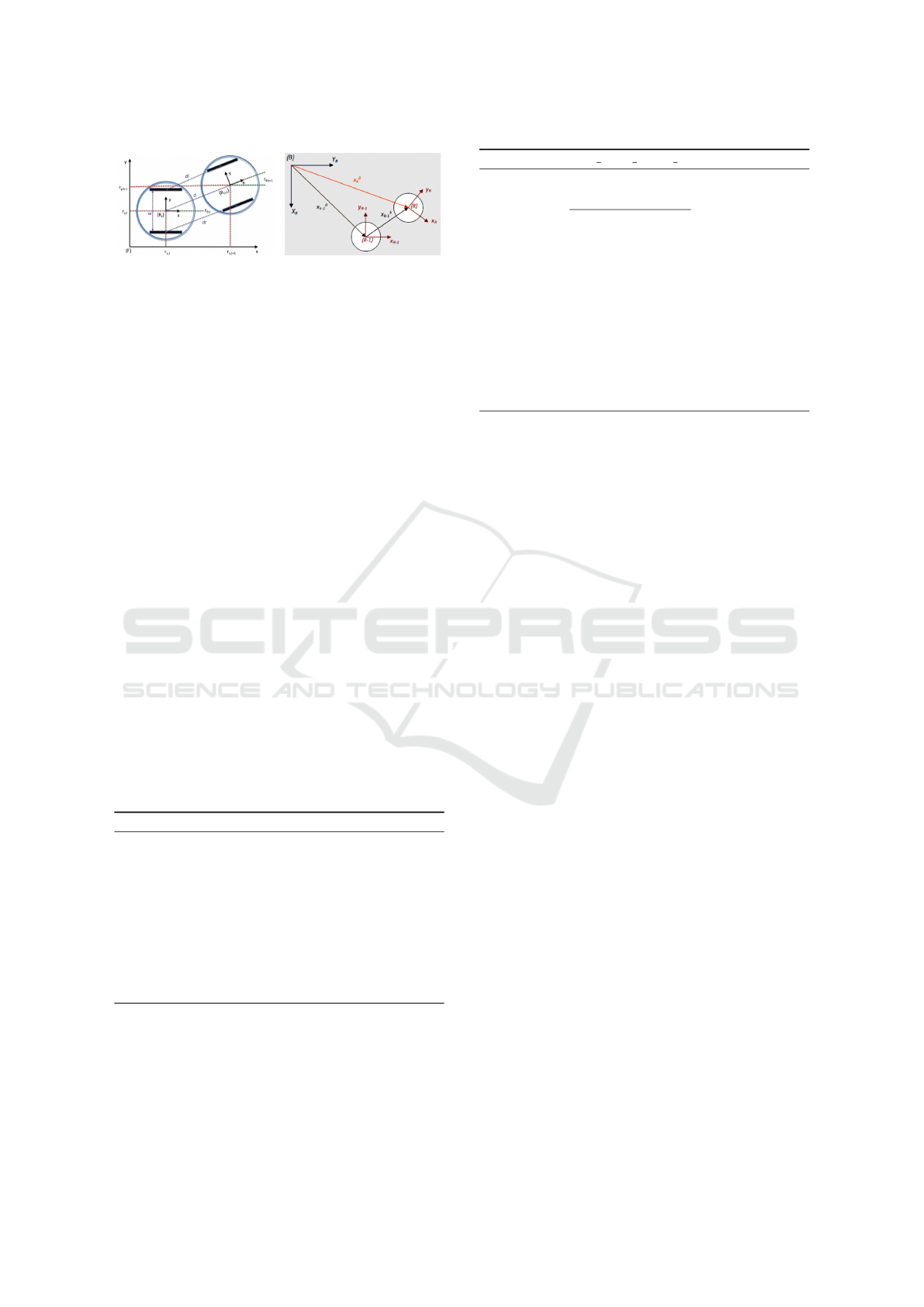
Figure 1: Left: The inexpensive e-puck mobile robot used
in the experiments. Middle: The model for odometry com-
putations in e-puck. Here, motion between two consecutive
time instants is show. Right: The model for rigid body
transformations for e-puck, based on position and heading
direction in two consecutive time instants.
step, the difference between the measured global po-
sition of the robot and the estimated global position
of the robot, z
k
− z
B
k
, was calculated. By these calcu-
lations, the mean x
k
and covariance P
k
were updated.
3.2 Occupancy Grid Mapping
Occupancy Grid Mapping (OGM) has become one
of the dominant paradigms for environmental model-
ing in mobile robotics (P. Schmuck and Zell, 2016;
Colleens and Colleens, 2007; D. Kortenkamp and
Murphy, 1998). OGM addresses the mapping prob-
lem under the assumption that the robot pose is
known. A 2D floor plan OGM map describes a 2D
slice of the 3D world. The basic idea was to represent
the map as a field of random variables known as cells,
arranged in an evenly spaced grid. Each cell in the
2D grid contained quantitative information regarding
the environment. OGM algorithm updates the poste-
rior over each grid cell as being occupied, empty or
unknown (Elfes, 1989) based on approximate poste-
rior estimation. The implemented mapping algorithm
updated the cells based on inverse sensor model algo-
rithm (S. Thrun and Fox, 2005).
Algorithm 2: Occupancy Grid Mapping.
1: procedure OGM({l
t−1,i
},x
t
,z
t
)
2: for all cells m
i
do
3: if m
i
in perceptual field of z
i
then
4: l
t,i
= l
t−1,i
+IRSM (m
i
,x
t
,z
t
) −l
0
5: else
6: l
t,i
= l
t−1,i
7: endif
8: endfor
9: return (l
t,i
)
OGM used log odds for the representation of oc-
cupancy. The odds of a state x were defined as the
ratio of the probability of that event divided by the
probability of its complement. The advantage of log-
odds over the probability representation was that they
can avoid numerical instabilities for probabilities near
Algorithm 3: inverse range sensor model.
1: procedure IRSM(i,x
t
,z
t
)
2: let x
i
,y
i
be the center of mass of m
i
3: r =
p
(x
i
− x)
2
+ (y
i
− y)
2
4: φ = atan2(y
i
− y,x
i
− x) − θ
5: k = argmin
j
|φ − θ
j,sens
|
6: if r > min(z
max
,z
k
t
+ α/2) or |φ − θ
j,sens
| >
β/2 then
7: return l
0
8: if z
k
< z
max
and|r − z
max
| < α/2
9: return l
occ
10: if r ≤ z
k
t
11: return l
f ree
12: endif
zero and one. The algorithm had previous log-odds
l
t−1
, current robot pose x
t
and measurement z
t
as in-
put. It looped through all grid cells and updated those
cells, which fall into the sensor cone of the measured
z
t
. The update of the occupancy log-odds value was
done by using the inverse range sensor model algo-
rithm. The constant l
0
is the prior of occupancy rep-
resented as a log-odds ratio.
The inverse sensor model used for IR range sen-
sors assigned an occupancy value l
occ
to all the cells
inside the measurement cone. The width of the oc-
cupied region was controlled by the value α and the
opening angle of the sensor beam was given by β. The
inverse model first calculated the beam index k and
the range r for the center of mass of the cell m
i
. The
prior for occupancy in log-odds form l
0
was returned
if the cell was outside the measurement cone or if it
lied more than α/2 distance behind the detected range
z
t
. It returned l
occ
if the range of the cell was within
α/2 of the detected range z
t
. It returned l
f ree
range
of the cell was shorter than the measurement range by
more than α/2.
3.3 Monte-Carlo Localization
Monte Carlo Localization (MCL) represents the pos-
terior using a particle set, which makes it a non para-
metric implementation of the Bayes filter. Being non-
parametric, it can represent a much broader space
of distributions. Each particle is an instance of the
state at time t, which is a hypothesis of the actual
state. The measurement model assigns weights the
estimated particles hypotheses making sure of the sur-
vival of the particles closer to the true state. The se-
lection of an appropriate measurement model is an
important step.
The MCL algorithm was obtained by substituting
the appropriate probabilistic motion model and mea-
surement model in the particle filter algorithm. The
Localization and Mapping of Cheap Educational Robot with Low Bandwidth Noisy IR Sensors
585

Algorithm 4: Monte-Carlo Localization.
1: procedure MCL(χ
t−1
,u
t
,z
t
,m)
2:
¯
χ
t
= χ
t
=
/
0
3: for m = 1 to M do
4: x
[m]
t
= sample motion model(u
t
,x
[m]
t−1
)
5: w
[m]
i
= measurement model(z
t
,x
[m]
t
,m)
6:
¯
χ
t
=
¯
χ
t
+ < x
[m]
t
,w
[m]
t
>
7: endfor
8: for m = 1 to M do
9: draw i with probability ∝ w
[i]
t
10: add x
[i]
t
toχ
t
11: endfor
12: return χ
t
inputs of the algorithm were a particle set χ
t−1
, odom-
etry u
t
, the most recent measurement z
t
and an oc-
cupancy grid map m of the environment. The algo-
rithm represents the belief bel(x
t
) as a set of M par-
ticles χ
t
= x
[1]
t
,x
[2]
t
,....,x
[M]
t
. Each particle x
t
was an
instance of the state at time t, which was a hypothe-
sis of the actual state. The state transition probability
density p(x
t
|x
t−1
,u
t
) was updated by using a sample
motion model. Then, the importance factor, w
[m]
t
for
each particle x
[m]
t
was calculated. The importance fac-
tor incorporates the measurement z
t
in the particle set
χ
t
. It calculated the probability of measurement z
t
under the updated particle set χ
t
. The predicted parti-
cle set and the normalized measurement weights were
then used to resample the particle set through impor-
tance resampling. Here, the probability of drawing
each particle was given by its importance weight. The
three most important steps of the algorithm were sam-
ple motion model, measurement model and the im-
portance resampling algorithm. The sample motion
model incorporated the motion u
t
of every particle in
the particle set. Each particle was updated with some
different random noise to model the uncertainty of the
environment. The importance resampling step made
use of the low variance sampler (S. Thrun and Fox,
2005). The measurement motion model used in this
application was the correlation based sensor models.
4 EXPERIMENTAL SETUP
To conduct the experiments of the above mentioned
algorithms, we used an 800mm by 600mm 2D
wooden field, an overhead camera covering the whole
field in its field of view (FOV) and an educational mo-
bile robot, e-puck.
The 2D rectangular field was placed in the labo-
ratory where ample ambient light was present in the
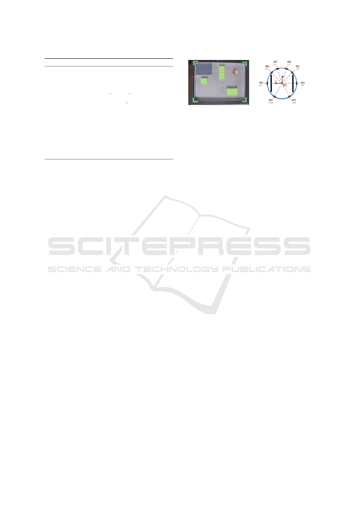
Figure 2: Left: A 2D planar field with e-puck mobile robot.
Global coordinate frame in Orange and Robot coordinate
frame in Blue. The checkers board calibration patten for
extrinsic parameters in on the arena as well. Middle: The
orientation of IR sensors on the e-puck is shown. Right:
The e-puck robot in the arena with its IR rays extended upto
6cms.
surroundings, shown in Figure. 2. The area encom-
passed by the field can be identified with four ’L’
shaped dark green markers pasted on each corner of
the field. While moving around the field, the robot
could encounter two types of walls. The wall of ob-
stacles (OW), which had green markers on top and
the boundary walls of the field (FW). Both types of
walls were painted white so that maximum Infrared
rays could get reflected off them. The size of obsta-
cles was greater than the size of the robot. The field
was relatively small and movable.
The overhead camera was a SONY SSC-DC198P
and it was fixed on top of the field. The calibration of
the camera was done by using Faugeras-Tosconi pin-
hole model, implemented in Matlab’s Camera Cali-
bration Toolbox. In total, 18 checker board images in
various orientations were used to get the intrinsic pa-
rameters. The extrinsic matrix was calculated by us-
ing the already calculated intrinsic parameters and the
checker board’s image placed beside the global origin
of the field as shown in Figure. 2. As the field was
movable, the extrinsic matrix had to be re-calculated
before the start of operation each time.
The mobile robot used for experimentation was
e-puck, which was a small, cheap and resourceful
(F. Mondada and Martinoli, 2009). Overall three ba-
sic utilities of e-puck were used: motors for motion,
encoders for odometry and Infrared Range (IR) sen-
sors for range sensing. Throughout the experiment,
the two stepper motors of the robot were moved with
constant linear and angular velocity. The encoder
pulse count of each wheel, when calculated with the
wheel circumference and axle length, gave an esti-
mate of the robot pose in the robot’s coordinate frame.
This estimation of pose is known as odometry, u
k
.
The 8 IR sensors, orientations shown in Figure. 2,
present on e-puck were used to calculate the distance
of obstacles from the robot. The effective range of
these IR sensors was a maximum of 6 cm with a very
narrow opening angle. This meant that an IR sensor
ICPRAM 2017 - 6th International Conference on Pattern Recognition Applications and Methods
586

detects an obstacle only when the IR beam was almost
perpendicular to the obstacle.
4.1 Results
Dataset. To be able to work offline, a dataset of
e-puck’s motion around the field was created storing
all the desired variables. The path followed by the
robot covered the whole field many times so that
there was enough data for validation as well. For
the implementation of each algorithm, the desired
variables were taken from the dataset and evaluated.
EKF Localization. The center of the field was taken
to be the initial belief with uncertainty in the covari-
ance matrix covering the whole arena shown in Fig-
ure. 3. The prediction step took into account the
odometry control input. The mean of belief was up-
dated by compounding the computed odometry with
the previous belief. The compounding function was
a non linear function, which also had noise affect
catered in it.
For every iteration in the measurement step, an
image was taken by the camera and processed using
the calibration parameters to identify the robot pose
with respect to the global coordinate frame. The
algorithm performed color segmentation and then
calculated the centroid of the robot. This estimated
robot pose, with its associated covariance matrix,
was then used to update the robot position mean and
covariance. Colored semi-circular markers were used
to determine the orientation (heading direction), of
the robot. In this case, where an overhead camera was
used for measurement, the measurement equation
was formulated by a linear equation. The update step
was performed by using the mean and covariance
generated in the prediction step in conjunction with
the measurement and measurement noise. The update
strengthens the robot belief around the true robot
pose shown in Figure. 3. Three iterations 1st, 16th
and 76th are shown in the figure. It can be seen
that as the number of iteration increases, the robot
belief strengthens around its true location. It can be
visually verified that with the increase in the number
of iterations, the Gaussian of robot belief grows
narrower, showing that the robot is confident about its
estimated pose. If at any time the update is stopped,
the robot belief still follows the robot around but the
uncertainty region starts expanding with respect to
the standard deviation in odometry.
Occupancy Grid Mapping. Occupancy grid map of
the environment inside the field was created by using
the IR sensors on the mobile robot e-puck. The image
overlay of the map is shown on top of the images cap-
tured by the overhead camera. The measured range
from each IR sensor was mapped by using the OGM
algorithm to retrieve a local map. In the implemented
algorithm, the IR sensor readings were taken to be
deterministic, which means the measured light falling
on the receptor of the sensor was converted into dis-
tance and was taken as the true value of distance. This
was an extraordinary assumption and should be taken
care of in the future.
In the presented result, the grid cell size in the
software map was 1mm and the real size of the field
was 600 mm x 800 mm. The images representing
the results had the same pixel ratio, with walls of
the field extending from each side. That meant that
a pixel in the image corresponds to 1mm in distance.
When evaluating the sharpness of edges in the map,
this measure is very important. The robot was made
to move beside the obstacles in the free space around
the field several times in the collected dataset so that
enough data is available for the mapping step. The re-
sult showed that not all the walls of obstacles and the
field are updated, there are discontinuities present in
them. As the grid cell size was too small, the noise in
measurement affected the grid cell update a lot. This
will not be the case if the resolution is higher, as then
the measurement to noise ratio will differ.
In Figure. 5, the back converted log odds map, into
probability map, is shown. All the values in the map
fall between 0 and 1. There are three colors in gray
scale, which identify the different type of grid cells.
These can be identified visually, as gray color show-
ing the grid cells, which were not updated and are un-
knowns, the white colored grid cells representing the
obstacles and the black colored grid cells representing
the free space.
The result of OGM is shown on top of the ground
truth. In Figure. 5, left image, only the grid pixels
identified as occupied are plotted in white on top
of the image with one to one correspondence in
millimetre scale. It can be visually verified that the
image fits perfectly on top of the obstacles and the
boundary walls. In addition to the occupied cells,
the cells which were classified as unknowns are also
pasted on top of the ground truth in black color.
Although most of the cells were correctly classified,
there were other cells, which are actually free but
are classified as unknowns. This happens because
of the small opening angle of the IR beam. It can
easily be removed in a post processing step, where
all these cells in the field except for obstacles, would
be classified as free under the condition that a single
clot of unknown cells is smaller than the size of
the robot. This can only be done if the size of the
Localization and Mapping of Cheap Educational Robot with Low Bandwidth Noisy IR Sensors
587

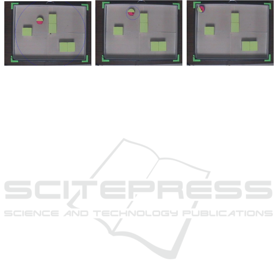
Figure 3: Left: The 1st iteration. The mean of initial belief of EKF is in the center of the field represented with a cross ’x’
and the covariance ellipse covers the whole field shown in ’blue circle’. Middle: The 16th iteration. The mean in the updated
belief is converging towards the true robot pose in subsequent iterations. Right:The 76th iteration. The belief grows even
more strong in the subsequent iterations. The covariance ellipse is smaller, which shows that the algorithm has converged.
obstacle is assumed to be greater than the size of the
robot, which was the case in our implementation.
The presented results are a good approximation of
the actual map.
Monte-Carlo Localization. Monte-Carlo localiza-
tion was implemented by using the occupancy grid
map generated by OGM and the IR sensors of the
e-puck. The inputs of the algorithm were a particle
set χ
t−1
, odometry control input u
t
, the most recent
measurement z
t
and an occupancy grid map m of the
environment. It first samples the motion model, then
calculates weights by measurement model and then
resamples the particle set.
In the resampling step, the low variance sampler
generates a single random number and selects sam-
ples according to this number but, still, with a prob-
ability proportional to the sample weight. The result
is a resampled particle set, with the density of particle
presence increased in the areas, where the particles
had more weight. A drawback of resampling is that
if it is done too often the diversity in the particle set
vanishes and if it is too infrequent, then the particle
samples are wasted in regions of low probabilities. A
rule of thumb to solve this problem is to check the
particle weight covariance, Neff, and resample, if it is
bigger than a threshold, Nth taken to be M/2.
In the presented results, the number of particles
M was 1000 so Nth was 500. In the first experiment,
resampling was done in every step and Neff was not
used. After just the first resampling step, it can be
seen in Figure. 4 that the particles beside the FW and
OW, whose local map intersected with obstacles on
the global map, got minimum weight and hence were
not resampled. This happens because in measurement
z
k
no obstacle was detected.
In the subsequent iterations, the robot kept on
moving along its path with particles oriented ran-
domly in the free space until an obstacle was detected.
In this case, after resampling, only the particles which
were oriented along FW or OW remain as in Figure. 4.
The robot moved along with the FW on its right side.
All the particles in the field moving in a pattern sim-
ilar to robot motion got equivalent weightage. As the
robot arrived closer to the wall perpendicular to it, this
act was another feature for localization. The parti-
cles, which do not agree with robot motion, start los-
ing weight and the accumulation of particles near the
true robot pose continued. Thus, eventually only one
belief is left which was in agreement with the true
robot pose, as can be seen by the covariance ellipse
of the particle cluster in Figure. 4. In all the subse-
quent robot motion, the mean, x, of particle cluster
remained close to the true robot belief with the error
being inside the 3σ bound as depicted in Figure. 7.
In the second type of results presented, Neff based
resampling was performed. This enabled diversity in
the particle set, without adding too many particles of
low probability. The algorithm was initialized in the
same manner with uniformly distributed random par-
ticles. When the weight covariance was less than a
threshold, the algorithm instead of resampling multi-
plied the recently calculated weights with the weights
of the previous step. This made sure that the parti-
cles with more plausible pose get more weight and
at the same time the particles with low probability
should not vanish in just one iteration. When the robot
approached the FW, the robot belief around the true
robot position strengthened. At the same time, other
plausible beliefs were also kept. This was the major
difference in Neff based MCL that it keeps a track
of all the possible beliefs till very late, shown in Fig-
ure. 6. As the robot approached further unique posi-
tions near both, the FW or the OW, the belief around
the true robot position grew until all the other hy-
potheses disappear, and all the particles converge to
the true robot belief shown in Figure. 6.
It should be noticed that in Figure. 6, it is the 201
iteration of the robot motion sequence. It is very dif-
ferent in comparison with results presented for the
ICPRAM 2017 - 6th International Conference on Pattern Recognition Applications and Methods
588

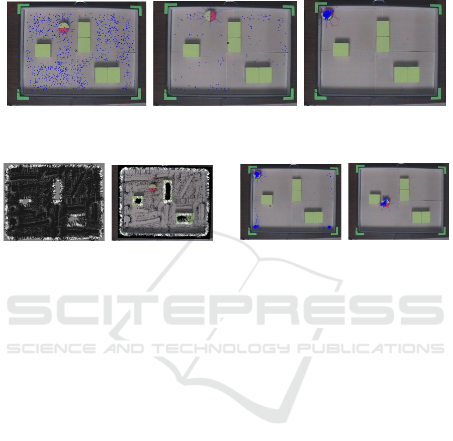
Figure 4: These results are without Neff. Left: MCL result in 1st iteration. MCl is initialized with particles randomly
oriented. Middle: The 21st iteration. The particles resample. The particles are not converging because of the self similariy of
the arena. Right: The 76th iteration. MCL is converging, as along the walls and then around the corner, the self similarity is
minimum and the particles converge.
Figure 5: Left: Occupancy Grid Map of the environment
shown in grayscale, with white showing the obstacles, black
representing the free cells and gray color showing the un-
known parts of the field. Right: Occupancy Grid Map reg-
istered on top of the ground truth with obstacles in white and
unknowns in black. It is a 1 to 1 scale mapping between the
arena area and the IR sensed distances, in millimeters.
first experiment, where the robot had converged even
in the 80
th
iteration. This result gives a good idea as
to how important it to consider weight covariance for
making a decision about resampling. It makes sure
that all the different hypotheses generated by the par-
ticle set are given their due importance until it sub-
stantially establishes the most suitable one. This kind
of particle diversity is important in self similar envi-
ronments like the one being considered for these ex-
periments. Here again in all the subsequent robot mo-
tion, the mean, x, of particle cluster remains close to
the true robot belief with the error being inside the 3σ
bound as depicted in Figure. 7.
The error in x and y coordinates of the ground truth
against the particle cluster mean is shown in Figure. 7.
One set of results is without Neff and one with it. It
can be seen that when Neff is used, the particles fol-
low the ground truth more steadily, with less error in
each axis. In both cases, the error in estimation is
bounded by 3σ range but the change in standard devi-
ation is not as rapid in Neff as it is without it, which
makes the use of Neff more desirable.
Figure 6: These results are with Neff. Left: MCL result
with Neff in 80
th
iteration, which is very different from the
one shown earlier in Figure. 4. Right: MCL result with
Neff in 201st iteration. This is when the particle set has
converged to the true robot belief, much later than the one
without Neff.
5 DISCUSSION
The presented results were attained with the limited
resources of the educational e-puck robot. The robot
had two limitations regarding range sensing. The first
is that the field of view in range sensing was limited
as IR sensors have a very narrow beam of measure-
ment and there were no other range sensors avail-
able. The second limitation was that the accuracy in
IR range sensing is not good because it is easily tem-
pered by ambient light. This makes the conversion of
light reading into distance inconsistent, which makes
the whole mapping and localization problem unreli-
able. Another drawback is that IR sensors only detect
an obstacle when the obstacle wall is almost perpen-
dicular to the IR beam. This means that even when
an obstacle is present in the IR sensor measurement
range, it does not detect it because the beam is not
perpendicular. This makes the sensor measurement
more unreliable and makes the localization problem
that much more difficult. Nonetheless, it can be seen
that even in the presence of noise, and low cost IR
sensors, the robot was able to localize itself in an un-
known environment. It is definitely a leap in terms of
the development of educational robots.
Localization and Mapping of Cheap Educational Robot with Low Bandwidth Noisy IR Sensors
589

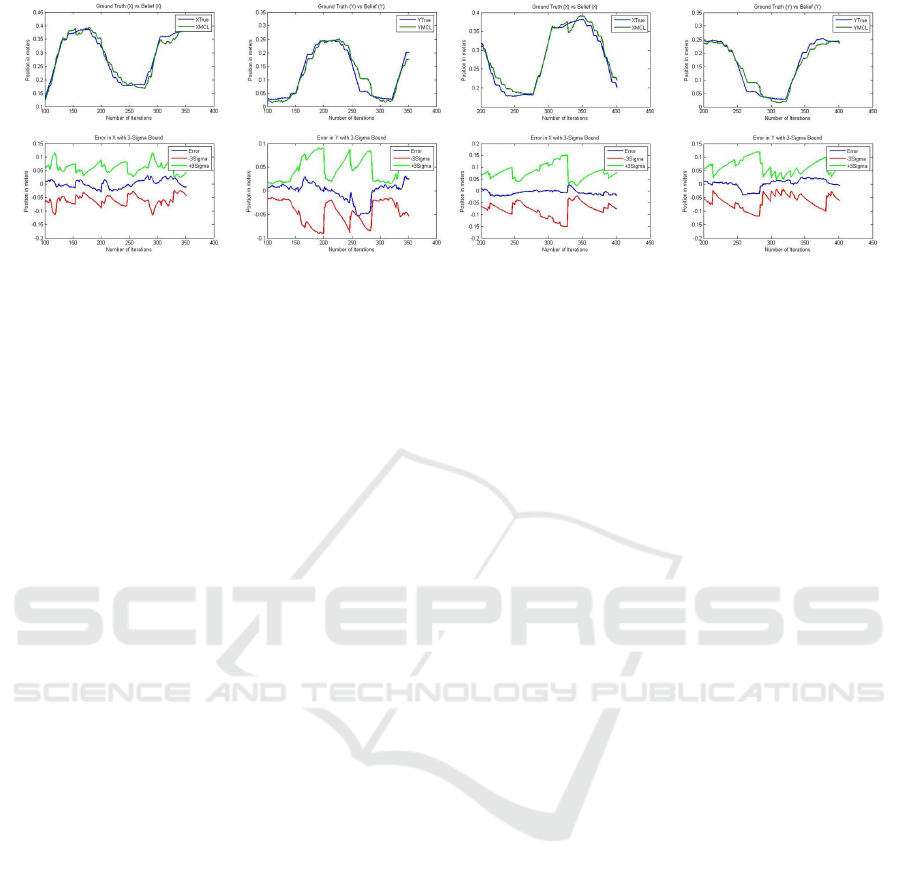
Figure 7: Each column pair contains (x, y) position of the robot. Left two columns: Error with 3σ bound without Neff. Right
two Column: Error with 3σ bound with Neff.
6 CONCLUSIONS
The work presented in this paper showed an inexpen-
sive educational robots with low cost noisy sensors
being used to demonstrate complex localization and
mapping concepts. We were able to implement and
demonstrate different techniques of solving two of the
major problems of mobile robotics i.e. Localization
and Mapping. The methods implemented were EKF
Localization, Occupancy Grid Mapping and MCL. In
the paper, it was demonstrated that these complex al-
gorithms can be implemented in a real environment
with a cheap robot. A natural progression of our work
is the implementation of the Simultaneous Localiza-
tion and Mapping (SLAM) problem on such plat-
forms. More specifically, the compiled dataset and
the implementation results acquired in this paper are
very useful to be used in more advanced algorithms,
i.e. Occupancy Grid based FastSLAM or DP-SLAM
among others. In general, our contribution enhances
the usage of small educational robots to demonstrate
complex robotics concepts.
REFERENCES
A. Prorok, A. B. and Martinoli, A. (2012). Low-cost col-
laborative localization for large-scale multi-robot sys-
tems. In Robotics and Automation (ICRA), 2012 IEEE
International Conference on. IEEE.
A.D. Cucci, M. Migliavacca, A. B. and Matteucci, M.
(2016). Development of mobile robots using off-
the-shelf open-source hardware and software compo-
nents for motion and pose tracking. In Intelligent Au-
tonomous Systems. SPRINGER.
Ahmad, H. and Namerikawa, T. (2010). Robot localiza-
tion and mapping problem with unknown noise char-
acteristics. In 2010 IEEE International Conference on
Control Applications. IEEE.
C. Sprunk, J. R
¨
owek
¨
amper, G. P. L. S. G. T. W. B. and
Jalobeanu, M. (2016). An experimental protocol for
benchmarking robotic indoor navigation. In Experi-
mental Robotics. SPRINGER.
Colleens, T. and Colleens, J. (2007). Occupancy grid map-
ping: An empirical evaluation. In Mediterranean
Conference on Control & Automation. IEEE.
D. Kortenkamp, R. B. and Murphy, R. (1998). Ai-based
mobile robots: Case studies of successful robot sys-
tems. CAMBRIDGE.
Elfes, A. (1989). Occupancy grids: A probabilistic frame-
work for robot perception and navigation. CMU.
F. Mondada, M. Bonani, X. R. J. P. C. C. A. K. S. M. J. Z.
D. F. and Martinoli, A. (2009). The e-puck, a robot de-
signed for education in engineering. In conference on
autonomous robot systems and competitions. IPCB.
J. McLurkin, A. Lynch, J. A. S. R. T. B. A. C. K. F. and
Bilstein, S. (2013). A low-cost multi-robot system for
research, teaching, and outreach. In Distributed Au-
tonomous Robotic Systems. SPRINGER.
M. Markom, A. Adom, E. T. S. S. A. R. and Shakaff, M.
(2015). A mapping mobile robot using rp lidar scan-
ner. In International Symposium on Robotics and In-
telligent Sensors. IEEE.
P. Schmuck, S. S. and Zell, A. (2016). Hybrid metric-
topological 3d occupancy grid maps for large-scale
mapping. In IFAC-PapersOnLine. ELSEVIER.
S. Bazeille, E. B. and Filliat, D. (2015). A light visual map-
ping and navigation framework for low-cost robots. In
Journal of Intelligent Systems. DE GRUYTER.
S. Thrun, W. B. and Fox, D. (2005). Probabilistic Robotics.
MIT Press, USA, 2nd edition.
S. Wang, F.Colas, M. L. F. M. and Magnenat, S. (2016). Lo-
calization of inexpensive robots with low-bandwidth
sensors. In 13th International Symposium on Dis-
tributed Autonomous Robotic Systems. INRIA.
Shim, J. and Cho, Y. (2016). A mobile robot localization via
indoor fixed remote surveillance cameras. In Sensors.
MDPI.
Tribelhorn, B. and Dodds, Z. (2007). Evaluating the
roomba: A low-cost, ubiquitous platform for robotics
research and education. In International Conference
on Robotics and Automation. IEEE.
ICPRAM 2017 - 6th International Conference on Pattern Recognition Applications and Methods
590