Three-dimensional Object Recognition via Subspace Representation
on a Grassmann Manifold
Ryoma Yataka and Kazuhiro Fukui
Graduate School of Systems and Information Engineering, University of Tsukuba,
1-1-1 Tennodai, Tsukuba, Ibaraki 305-8573, Japan
Keywords:
Three-dimensional Object Recognition, Subspace Representation, Canonical Angles, Grassmann Manifold,
Mutual Subspace Method.
Abstract:
In this paper, we propose a method for recognizing three-dimensional (3D) objects using multi-view depth
images. To derive the essential 3D shape information extracted from these images for stable and accurate 3D
object recognition, we need to consider how to integrate partial shapes of a 3D object. To address this issue,
we introduce two ideas. The first idea is to represent a partial shape of the 3D object by a three-dimensional
subspace in a high-dimensional vector space. The second idea is to represent a set of the shape subspaces as
a subspace on a Grassmann manifold, which reflects the 3D shape of the object more completely. Further,
we measure the similarity between two subspaces on the Grassmann manifold by using the canonical angles
between them. This measurement enables us to construct a more stable and accurate method based on richer
information about the 3D shape. We refer to this method based on subspaces on a Grassmann manifold as the
Grassmann mutual subspace method (GMSM). To further enhance the performance of the GMSM, we equip
it with powerful feature-extraction capabilities. The validity of the proposed method is demonstrated through
experimental comparisons with several conventional methods on a hand-depth image dataset.
1 INTRODUCTION
Depth images represent a very informative resource
with which to construct a method for recognizing
three-dimensional (3D) objects. Because it is now rel-
atively easy to capture depth images, many methods
using either individual depth images or depth image
sets have been proposed (Dreuw et al., 2009; Jian-
guo et al., 2010; Jamie et al., 2012; Shen et al., 2012;
Yu et al., 2014; Song and Xiao, 2014; Stefania et al.,
2014; Watanabe et al., 2014). In this paper, we dis-
cuss a method for recognizing 3D objects from multi-
view depth images. This method is based on subspace
representation with a Grassmann manifold.
The proposed method is motivated by the con-
cept of a shape subspace, which can compactly rep-
resent the geometrical structure of a set of feature
points from a 3D object (Kanade et al., 1997). Be-
cause the shape subspace concept is simple and scal-
able, it has been used in various recognition methods,
such as an identification method based on the geomet-
rical structure of micro-facial-feature points (Yosuke
and Kazuhiro, 2011; Yoshinuma et al., 2015). Shape
subspaces were originally generated from sequential
images as a byproduct of the factorization method
(Tomasi and Kanade, 1992). In this paper, we gen-
erate a shape subspace directly from a depth image
by sampling 3D points randomly from its 3D surface
mesh.
To realize more stable and accurate 3D object
recognition with multi-view depth images, we need to
integrate the partial shapes from multi-view depth im-
ages into a more complete 3D shape. This is because
each depth image can capture only part of the shape
of the 3D object. In our setting, we need to consider
how to integrate a set of shape subspaces into one rep-
resentational form.
To address the above integration problem, we fo-
cus on methods based on image sets, which have
been attracting much attention in the field of computer
vision. In particular, the mutual subspace method
(MSM) (Yamaguchi et al., 1998) is a well-known and
useful image-set-based method. The essence of the
MSM is to represent a set of images as a subspace
in a high-dimensional vector space (Lee et al., 2005;
Ronen and David, 2003). Once two sets of images are
represented as two subspaces, we can easily measure
the similarity between two sets by using the canonical
208
Yataka, R. and Fukui, K.
Three-dimensional Object Recognition via Subspace Representation on a Grassmann Manifold.
DOI: 10.5220/0006204702080216
In Proceedings of the 6th International Conference on Pattern Recognition Applications and Methods (ICPRAM 2017), pages 208-216
ISBN: 978-989-758-222-6
Copyright
c
 2017 by SCITEPRESS – Science and Technology Publications, Lda. All rights reserved

angles between the two corresponding subspaces.
To incorporate this idea of subspace representa-
tion into our problem for sets of shape subspaces, we
introduce the concept of a Grassmann manifold, in
which a shape subspace is represented by a point on
the Grassmann manifold. Although it is complicated
to operate directly on data on a Grassmann manifold,
embedding the Grassmann manifold into a reproduc-
ing kernel Hilbert space by using a Grassmann ker-
nel makes the operation easier to implement. In this
case, we can apply kernel principal component anal-
ysis (PCA) with a Grassmann kernel to a set of shape
subspaces as we would for a usual vector space, and
we refer to this PCA as Grassmann PCA (GPCA).
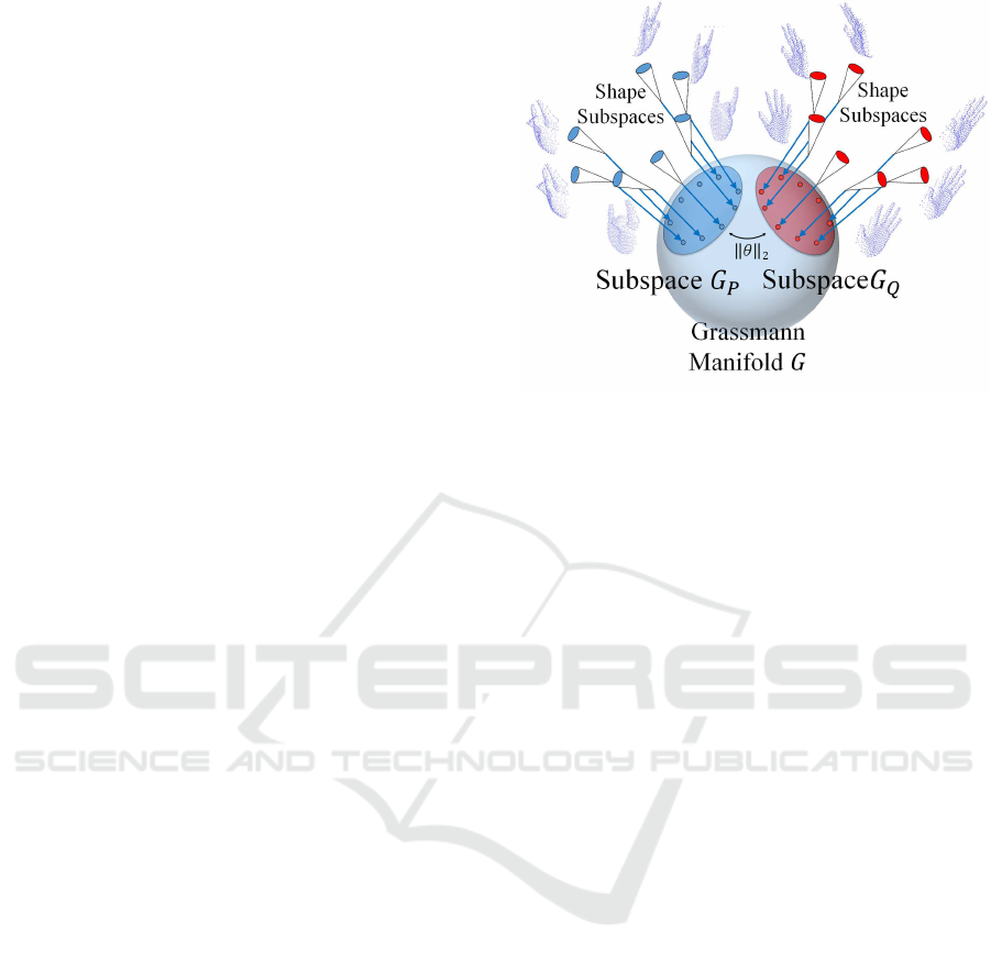
The details of this process will be described later. Fig-
ure 1 shows a conceptual diagram of our subspace
representation on a Grassmann manifold, where two
sets of shape subspaces are represented by subspaces
G
P
and G
Q
, respectively. These subspaces reflect
more complete 3D shapes of the two types of hand
shape.
Furthermore, we measure the similarity between
G
P
and G
Q
on the Grassmann manifold by using the
canonical angles between them. This measurement
enables us to construct a more stable and accurate
method with richer information about a more com-
plete 3D shape.
We refer to this extension of MSM on a Grass-
mann manifold as the Grassmann mutual subspace
method (GMSM). Mutual subspace methods have
been extended to the constraint MSM (CMSM)
(Fukui and Yamaguchi, 2003) and orthogonal MSM
(OMSM) (Kawahara et al., 2007) by incorporating
powerful feature extractions. Motivated by these ex-
tensions, we construct the CMSM and OMSM on a
Grassmann manifold and refer to them as GCMSM
and GOMSM, respectively.
The main contributions of this paper are summa-
rized as follows.
1) We introduce a method for generating a shape
subspace from a depth image.
2) We propose a method for integrating multiple
shape subspaces obtained at multi-view points by
introducing subspace representation on a Grass-
mann manifold.
3) We demonstrate the validity of the proposed
method through experiments with a dataset of
hand-shape depth images with 10 classes.
The rest of this paper is organized as follows. In
Section 2, we describe the basic idea of the proposed
method. In Section 3, we describe the details of the
proposed method, which is based on subspace repre-
sentation on a Grassmann manifold. In Section 4, we
Figure 1: Subspace representation on a Grassmann mani-
fold. By introducing this representation, a set of shape sub-
spaces can be represented compactly by a subspace on the
Grassmann manifold.
explain the algorithm of the proposed framework. In
Section 5, we present experiments with hand-shape
depth images and discuss the results. Section 6 con-
cludes the paper.
2 BASIC IDEA
Our basic idea is derived from the assumption that
the distribution of shape subspaces from multi-view
depth images of a 3D object represent its shape more
completely. Under this assumption, we integrate the
partial 3D shapes of the obtained shape subspaces into
one representational form for a more complete 3D
shape by using subspace representation on a Grass-
mann manifold.
2.1 Subspace Representation in Vector
Space
The integration of shape subspaces was motivated by
the success of the MSM in 3D object recognition, as
mentioned previously. The MSM is one of several
useful image set-recognition methods used for recog-
nizing various objects, such as faces and hands (Fukui
and Yamaguchi, 2003; Ohkawa and Fukui, 2012).
Figure 2 shows a conceptual diagram of the MSM.
The validity of the MSM is due to the fact that a
set of multi-view images of a 3D object can be rep-
resented compactly by a low-dimensional subspace
in a high-dimensional vector space. For example, a
set of frontal facial images of a certain person under
various illumination conditions is contained within a
Three-dimensional Object Recognition via Subspace Representation on a Grassmann Manifold
209

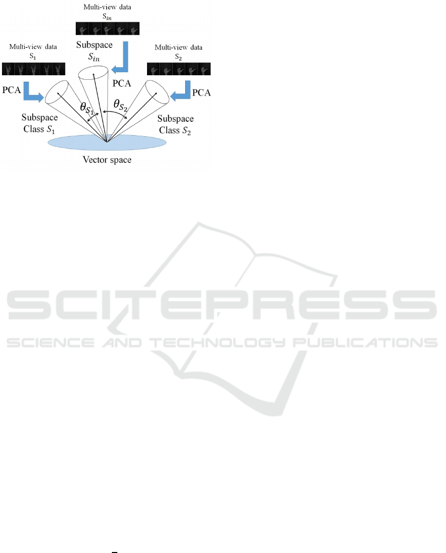
Figure 2: Conceptual diagram of MSM. This statistical clas-
sification method approximates patterns with subspaces by
using principal component analysis (PCA) to recognize in-
put patterns from canonical angles.
nine-dimensional subspace. Because the face direc-
tion may indeed change, the necessary dimensional-
ity may be higher than nine, but its upper limit is still
much lower than that of the original vector space.
The MSM classifies an input subspace by using
the canonical angles between the input and reference
subspaces. We now proceed to define a canonical an-
gle.
Given an n-dimensional shape subspace and an m-
dimensional shape subspace, where n ≤ m, the canon-
ical angle θ
i
(i = 1, . . . , n) is defined as
cos θ
i
= max
u
i
∈S
1
max
v
i
∈S
2
u
⊤
i
v
i
s.t.ku
i
k = kv
i
k = 1, u
⊤
i
v
j
= v
⊤
i
u
j
= 0. (1)
Several methods can be used to calculate canonical
angles (Maeda and Watanabe, 1985; Harold, 1936;
Afriat, 1957). Let Q
1
and Q
2
denote the respective
orthogonal projection matrices of subspaces S
1
and
S
2
; for instance, cos
2
θ
i
is the eigenvalue of Q
1
Q
2
or Q
2
Q
1
. The largest eigenvalue corresponds to the
smallest canonical angle θ
1
, and the second-largest
eigenvalue corresponds to the second-smallest canon-
ical angle θ
2
in a direction orthogonal to that of θ
1
.
The values cos
2
θ
i
(i = 3, . . . , n) are calculated simi-
larly. The similarity between two n-dimensional sub-
spaces S
1
and S
2
is defined as
sim(S
1
, S
2
) =
1
n
n
∑
i=1
cos
2
θ
i
. (2)
If two shape subspaces overlap completely, sim is
unity because all canonical angles are zero. In con-
trast, if two shape subspaces are orthogonal to each
other, sim is zero.
2.2 Subspace Representation on a
Grassmann Manifold
Our integration idea is based on the concept of a
Grassmann manifold. In our setting, the targets to be
considered are not vectors but shape subspaces. Nev-
ertheless, we expect that the validity of the subspace
representation used in the MSM can also work for
a set of shape subspaces on a Grassmann manifold,
thanks to the following useful characteristic.
Grassmann manifold G (m, D) is defined as a set
of m-dimensional linear subspaces in R
D
, where a
subspace in vector space R
D
is represented as one
point on the Grassmann manifold.
As we mentioned previously, to make our idea
easier to implement, we utilize the technique of em-
bedding a Grassmann manifold into a reproducing
kernel Hilbert space by using a Grassmann kernel
(Hamm and Lee, 2008). In this paper, we use the
projection kernel (Hamm and Lee, 2008) as a kernel
function, which is defined as follows:
k(S
1
, S
2
) = sim(S
1
, S
2
), (3)
where sim is that defined by Eq. (3).
We cannot operate on a shape subspace mapped
on the Grassmann manifold when using the kernel
trick with the Gaussian kernel. However, we can
calculate the inner product between two given points
(shape subspaces) on the manifold through the Grass-
mann kernel function.
The similarity between an input point (shape sub-
space S) and a reference point (shape subspace S
′
i
)
can be calculated as follows:
k (S) = k

S, S
′
i

. (4)
By using this relationship, we can apply PCA also
to a set of multiple points (shape subspaces) on the
Grassmann manifold as we would to a standard vec-
tor space.
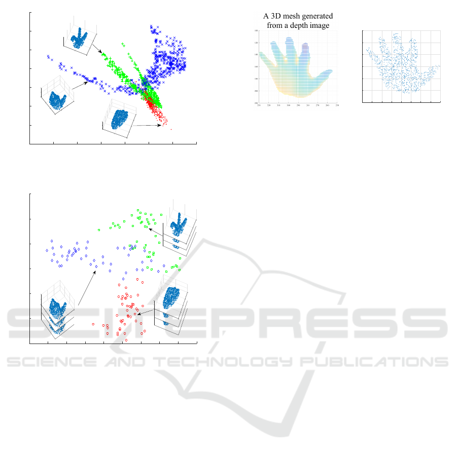
Figures 3 and 4 show the validity of the subspace
representation on a Grassmann manifold, where the
distributions of shape subspaces of three hand-shape
classes are visualized by using the multi-dimensional
scaling (MDS) (Michael and Trevor, 2008). In Fig. 3,
scatter map shows clearly the difficulty of distinguish-
ing the three classes. In contrast, Fig. 4 shows the
distributions of “subspaces” on the Grassmann mani-
fold, where each subspace was generated from a set of
multiple shape subspaces belonging to the same hand
class. These visualizations show that the subspace
representation improves the class separation signifi-
cantly.
ICPRAM 2017 - 6th International Conference on Pattern Recognition Applications and Methods
210

-5 -4 -3 -2 -1 0 1 2
-1.5
-1
-0.5
0
0.5
1
1.5
2
-100
-50
50
0
0
50
-50
-40
-20
0
100
50
20
0
40
-50
0
-100
50
40
-100
20
-50
0
0
-20
50
0
-50
Figure 3: Distribution of shape subspaces (points) on the
Grassmann manifold.
-2.5 -2 -1.5 -1 -0.5 0 0.5 1 1.5 2
-1.5
-1
-0.5
0
0.5
1
1.5
-40
-20
0
100
50
20
0
40
-50
0
-100
-100
-50
50
0
0
50
-50
50
40
-100
20
-50
0
0
-20
50
0
-50
Figure 4: Distribution of subspaces on the Grassmann man-
ifold, where each subspace was generated from a set of mul-
tiple shape subspaces belonging to the same class.
3 PROPOSED METHOD
In this section, we firstly describe the definition of
shape subspaces and how to generate them. We
then describe subspace representation on a Grass-
mann manifold in detail. Finally, we describe our
GMSM, GCMSM, and GOMSM algorithms.
3.1 Generation of Shape Subspace
A shape subspace is defined as a three-dimensional
subspace in a high-dimensional vector space. It is in-
variant under an affine transformation of the set of
feature points (Costeira and Kanade, 1998), such as
that caused by camera rotation or object motion. This
property is useful for 3D object recognition. Gener-
ally, shape subspaces are generated by applying the
factorization method (Tomasi and Kanade, 1992) to
sequential images. However, in our framework, we
-40-30-20-10010203040
-60
-40
-20
0
20
40
60
3D feature points
Figure 5: Random feature extraction. 3D feature points on
the 3D mesh are obtained from the depth image.
generate a shape subspace from a single depth image
by sampling 3D feature points randomly on the 3D
mesh that is obtained from the depth image (Fig. 5).
Assume that T 3D feature points were extracted
from a given depth image. In that case, shape sub-
space S would be spanned by the three column vec-
tors of a T × 3 matrix S that is defined as follows:
S = (s
1
, s
2
, . . . , s
T
)
⊤
=




x
1
y
1
z
1
x
2
y
2
z
2
.
.
.
.
.
.
.
.
.
x
T
y
T
z
T




, (5)
where s
p
= (x
p
, y
p
, z
p
)
⊤
(1 ≤ p ≤ T) denotes the po-
sitional vector of 3D feature point p.
3.2 Integration of Shape Subspaces on a
Grassmann Manifold
We integrate all the shape subspaces corresponding
to partial shapes into one subspace corresponding to
the whole shape by using the concept of a Grassmann
manifold. To achieve the integration, we apply PCA
to a set of shape subspaces mapped onto the Grass-
mann manifold.
The nonlinear function φ maps a three-
dimensional shape subspace S of R
T
onto a
subspace on the Grassmann manifold G(3, T),
φ : R
T
→ G(3, T), S → φ(S ). To perform PCA on
the mapped shape subspaces, we need to calculate the
inner product (φ(S
1
) · φ(S
2
)) between the function
values. We can calculate this through a kernel
function k(S
1
, S
2
). The PCA of the mapped shape
subspaces onto the Grassmann manifold is kernel
PCA with the Grassmann kernel (GPCA), and the
nonlinear subspace generated by doing so is the
subspace G
P
on the Grassmann manifold G(3, T).
Given G
k
P
of class k generated from L training
data S
k
l
(l = 1, . . . , L), the M orthonormal basis vectors
e
k
i
(i = 1, . . . , M), which span the subspace G
k
P
on the
Grassmann manifold, can be represented by a linear
Three-dimensional Object Recognition via Subspace Representation on a Grassmann Manifold
211

combination of φ(S
k
l
) as
e
k
i
=
L
∑
l=1
a
k
i,l
φ(S
k
l
). (6)
Here, the coefficient a
k
i,l
is the l-th component of the
eigenvector a
k
i
corresponding to the i-th largest eigen-
value λ
i
of the L×L Gram matrix K that is defined as
Ka = λa (7)
k
l,l
′
= (φ(S
k
l
) · φ(S
k
l
′
))
= k(S
k
l
, S
k
l
′
),
where a is normalized to satisfy λ(a · a) = 1. We use
the projection kernel from Eq. (4) as the kernel func-
tion. We can compute the projection of the mapped
φ(S) onto the i-th orthonormal basis vector
e
k
i
of the
subspace G
k
P
as
(φ(S),
e
k
i
) =
L
∑
l=1
a
k
i,l
k(S , S
k
l
). (8)
Assume that we obtain N orthogonal bases
u
i
(i = 1, 2, . . . , N) of subspace G
P
on the manifold
and M orthogonal bases
v
i
(i = 1, 2, . . . , M) of sub-
space G
Q
on the Grassmann manifold, where N ≤ M
by GPCA. In this case, the canonical angles θ
i
(i =
1, . . . , N) between subspaces G
P
and G
Q
can be cal-
culated as
cosθ
i
= max
u
i
∈G
P
max
v
i
∈G
Q
u
i
⊤
v
i
s.t.k
u
i
k = k
v
i
k = 1,
u
i
⊤
v
j
=
v
i
⊤
u
j
= 0. (9)
3.3 Grassmann MSM
The GMSM involves applying the MSM to two sub-
spaces on a Grassmann manifold given reference
multi-view shape subspaces S
k
l
(l = 1, . . . , N
k
) for each
class.
Training Phase
By applying GPCA to shape spaces S
k
l
for each
class, we generate reference subspaces G
k
P
on the
Grassmann manifold, the process of which was
described in Sec. 3.2.
Recognition Phase
1. By applying GPCA to input multi-view shape
spaces S
i
(i = 1, . . . , N
in
), we generate an input
subspace G
in
P
on the Grassmann manifold in the
same way as in the training phase.
2. We calculate the similarity defined as Eq. (11) be-
tween the input G
in
P
and each reference G
k
P
on the
Grassmann manifold.
3. The input G
in
P
is placed into the class with the
highest similarity.
3.4 Grassmann CMSM
The CMSM carries out the MSM using the class sub-
spaces that are mapped onto the constrained space
(Fukui and Yamaguchi, 2003). In the CMSM, a gen-
eralized difference subspace (GDS) (Fukui and Maki,
2015) is utilized as the constrained space; this sub-
space is obtained after deleting the common part of
all class subspaces. Therefore, we can enhance the
discriminatory ability by using the CMSM.
We construct the nonlinear kernel constrained mu-
tual subspace method (KCMSM) by applying the
MSM to the class subspaces that are mapped onto
the nonlinear constrained space. The GCMSM is the
KCMSM with the Grassmann kernel.
3.5 Grassmann OMSM
In the OMSM (Kawahara et al., 2007), firstly the class
subspaces are made orthogonal to each other and then
the MSM is applied to them. This orthogonalization
can enhance the discrimination ability of the MSM.
We construct the nonlinear kernel orthogonal mu-
tual subspace method (KOMSM) by applying the
MSM to the orthogonalized class subspaces. The
GOMSM is the KOMSM with the Grassmann kernel.
4 PROPOSED FRAMEWORK
FOR 3D OBJECT
RECOGNITION
In this section, we firstly describe the correspondence
process of feature points that we need to conduct be-
fore calculating the similarity between two shape sub-
spaces. Next, we explain the flow of the proposed
framework for 3D object recognition.
4.1 Correspondence of Feature Points
In our framework, although a shape subspace can be
generated as the column space of a matrix, as men-
tioned in Sec. 3.1, the shape subspace can change
when the order of its feature points changes. Thus,
we need to relate points between an input shape ma-
trix and a reference shape matrix before calculating
the similarity between the two corresponding shape
subspaces.
In this correspondence process, we use the first
input shape matrix S
1
as the reference. In other
words, the row elements of S
i
(i = 2, . . . , N
in
) and S
k
l
are sorted based on those of S
1
. For the correspon-
dence, we use the iterative closest point (ICP) algo-
ICPRAM 2017 - 6th International Conference on Pattern Recognition Applications and Methods
212

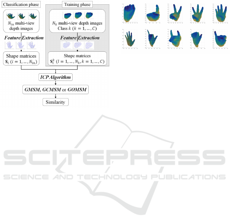
Figure 6: Diagram of proposed framework consisting of
training phase and classification phase.
rithm (Paul and Neil, 1992). Note that the above cor-
respondence process is needed in both the training
and classification phases.
4.2 Flow of the Proposed Framework
We consider the problem of classifying a whole in-
put shape that is represented by a set of multi-view
depth images into one of C shape classes. Figure 6
shows the diagram of proposed framework consisting
of training phase and classification phase. Given a set
of N
k
depth images for each class, the detailed process
is summarized as follows.
Training Phase
1. We extract the feature point sets from all refer-
ence multi-view depth images using the method
described in Sec. 3.1.
2. We set reference shape matrices S
k
l
(l =
1, . . . , N
k
;k = 1, . . . , C) as in Eq. (6).
Classification Phase
1. We extract the feature point sets from input multi-
view depth images in the same way as in the train-
ing phase.
2. We set the input shape matrices S
i
(i = 1, . . . , N
in
)
in the same way as in the training phase.
3. We conduct the correspondence process between
the input shape matrices S
i
and reference shape
matrices S
k
l
.
4. After completing the correspondence process, we
calculate class subspaces G
k
P
(k = 1, . . . , C) and an
Figure 7: Sample images of hand-shape data. These data
contain 10 categories.
input subspace G
in
P
by applying the algorithm of
the proposed method, that is, GMSM, GCMSM,
or GOMSM.
5. The input subspace G
in
P
is placed into the class
with the highest similarity.
5 EVALUATION EXPERIMENTS
ON HAND SHAPE
RECOGNITION
In this section, we demonstrate the validity of our
proposed method through two types of experiment
using the depth images of 10 hand-shape classes.
Firstly, we examined the characteristics of our sub-
space representation on a Grassmann manifold. Sec-
ondly, we conducted an experiment to evaluate the
proposed method in comparison with conventional
methods such as Grassmann discriminant analysis
(GDA) (Hamm and Lee, 2008), which is well known
as an effective classification method on Grassmann
manifolds.
5.1 Experimental Setup
We used a depth sensor (Microsoft Kinect v2) to cap-
ture 20 depth images of 5 subjects across 10 cat-
egories (5 × 20 × 10 = 1, 000 images) as shown in
Fig. 7. Each subject sat in a chair that was approxi-
mately 0.5 m away from the sensor. To capture multi-
view depth images, we asked each subject to rotate
their wrist in order to change the appearance of their
hand, as shown in Fig. 8. We cropped the hand re-
gion from each depth image and then extracted 1, 000
points randomly from the 3D mesh obtained of the
hand, as shown in Fig. 9.
5.2 Validity of Subspace Representation
Firstly, we examined the optimal dimensionality of
a subspace in which to represent a set of real hand-
Three-dimensional Object Recognition via Subspace Representation on a Grassmann Manifold
213

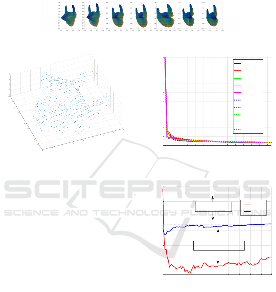
Figure 8: Samples of multi-view hand-shape images. The angle changes from zero to 70
◦
.
100
25
20
15
10
5
0
-5
-40
50
-30
-10
-20
-10
-15
0
10
-20
20
30
-25
40
0
-50
-100
Figure 9: Sample of the data points extracted from a depth
image. Each datum consists of 1, 000 feature points.
shape data. We generated 100 shape subspaces for
each class and then generated a subspace for each
class by applying GPCA to a set of the 100 shape sub-
spaces.
Figure 10 shows how the eigenvalue changes with
eigenvalue number; the vertical and horizontal axes
denote the eigenvalue and its order, respectively. This
indicates the representation ability of the generated
subspace. From this figure, we reason that a dimen-
sionality of 5 is sufficient for representing a set of
shape subspaces from the real hand-shape data.
Secondly, we evaluated the performances of the
proposed methods with subspace representation and
the MSM 1-nearest-neighbor (MSM-1NN) without
subspace representation while changing the dimen-
sionality of the class subspaces from 1 to 99. The
evaluation was done by using 100-fold cross valida-
tion, and the performances were measured in terms of
error rate (ER) and equal error rate (EER).
Figure 11 shows the experimental results of the
methods, where the vertical axis denotes the ER and
EER and the horizontal axis denotes the dimension
of the subspace on the Grassmann manifold. From
this graph, we can see that our proposed GMSM out-
performs the simple MSM-1NN in terms of ER and
EER, which means that our idea of subspace repre-
sentation on a Grassmann manifold works effectively
as expected.
1 3 5 7 9 11 13 15 17 19 21 23 25 27
Eigenvalue number
0
2
4
6
8
10
12
14
16
18
20
Eivenvalue
Distribution of eigenvalue
class 1
class 2
class 3
class 4
class 5
class 6
class 7
class 8
class 9
class 10
Figure 10: Distribution of eigenvalues when applying
GPCA for each hand.
1 10 20 30 40 50 60 70 80 90 99
Dimension
0.12
0.14
0.16
0.18
0.2
0.22
0.24
ER, EER
ER
EER
Proposed method
MSM-1NN
Figure 11: Classification accuracies of GMSM and MSM-
1MM for different subspace dimensionalities on a Grass-
mann manifold.
5.3 Experimental Comparison of
Proposed and Conventional
Methods
To verify the effectiveness of the proposed method,
we conducted a comparative experiment between our
proposed methods (GMSM, GCMSM, and GOMSM)
and the conventional methods (MSM-1NN and GDA-
ICPRAM 2017 - 6th International Conference on Pattern Recognition Applications and Methods
214

Table 1: Dimensionalities of test, reference, and constraint
subspaces for the different methods.
Reference Test Constraint
GMSM 30 8 -
GOMSM 30 8 -
GCMSM 30 8 480
1NN).
The evaluation procedure is summarized as fol-
lows: 1) We divided the 100 sequential shape sub-
spaces into the 10 data sets, which a set has 10 se-
quential shape subspaces. A data set and the remain-
ing 9 data sets used for training and for testing, re-
spectively; 2) To increase the number of trials, we
generated 91 test subsets of 10 shape subspaces by
sliding the window one by one over the 90 test shape
subspace. The total number of trial evaluations was
910 (= 91 test subsets ×10 classes). We repeat 1) and
2) ten times by changing the training data set. The av-
erage and the standard deviation (SD) of the ERs and
EERs of the 10 trials were used as the final evaluation
indexes.
In the proposed methods, we generated a test sub-
space from the 10 shape subspaces and a reference
subspace from the remaining 90 shape subspaces for
each class. In contrast, in the conventional methods,
an input is not a set of shape subspaces but rather an
individual single-shape subspace. Thus, in order to
perform a fair evaluation, we defined a new similarity
for the conventional methods between a test subset
and a reference set in terms of the mean of the 100
similarities in the combinations of 10 testing and 10
training shape subspaces. The dimensions of the test
and reference subspaces were decided by a prelimi-
nary experiment, as shown in Table 1.
Table 2 shows the evaluation results of all the
methods. Firstly, we can see that GMSM, GCMSM,
and GOMSM perform better in comparison with the
simple MSM-1NN that does not use subspace repre-
sentation on a Grassmann manifold. Secondly, we can
see that GMSM outperforms MSM-1NN appreciably,
meaning that our idea for subspace representation is
also valid for a set of shape subspaces on a Grass-
mann manifold, in the same way as in a vector space.
Thirdly, GCMSM and GOMSM perform better than
GMSM. This means that the feature extraction us-
ing GDS projection and the orthogonalization of class
subspaces also work on a Grassmann manifold, as
they do in a vector space. Finally, the performance
of GCMSM is comparable to that of GDA-1NN. This
suggests that the GDS projection has a similar dis-
criminative effect to that of Fisher discriminant anal-
ysis, which is used in GDA.
Table 2: Performances of all the methods in terms of ER
and EER.
ER (%) ± SD EER (%) ± SD
MSM-1NN 29.62± 1.01 27.00± 0.85
GDA-1NN 7.89± 0.90 5.32± 0.44
GMSM 7.85± 1.55 20.26± 0.86
GCMSM 9.19± 1.23 4.49± 0.59
GOMSM 8.47± 1.25 4.47± 0.45
6 CONCLUSIONS
In this paper, we proposed a novel method for 3D ob-
ject recognition based on subspace representation on a
Grassmann manifold. The main ideas of the proposed
method were 1) to represent a partial shape from some
viewpoint by a shape subspace in a high-dimensional
vector space; 2) to integrate all the shape subspaces
corresponding to partial shapes into a subspace corre-
sponding to the whole shape on the Grassmann man-
ifold; 3) to measure the similarity between the shape
subspaces.
The main purposes of this paper were 1) to pro-
pose a novel framework for subspace representation
on a Grassmann manifold and 2) to verify that it is
effective for 3D object recognition using multi-view
depth images. As expected, we were able to demon-
strate the basic effectiveness of subspace representa-
tion on a Grassmann manifold through comparison
experiments using a database of hand depth images.
However, to confirm the performances of the pro-
posed methods in more detail, we need to conduct
experiments with larger datasets.
ACKNOWLEDGEMENTS
Part of this work was supported by JSPS KAKENHI
Grant Number JP16H02842.
REFERENCES
Afriat, S. N. (1957). Orthogonal and oblique projectors and
the characteristics of pairs of vector spaces. Proceed-
ings of the Cambridge Philosophical Society, 53:800–
816.
Costeira, Jo˜ao, P. and Kanade, T. (1998). A multibody fac-
torization method for independently moving objects.
International Journal of Computer Vision, 29(3):159–
179.
Dreuw, P., Steingrube, P., Deselaers, T., and Ney, H. (2009).
Smoothed Disparity Maps for Continuous American
Three-dimensional Object Recognition via Subspace Representation on a Grassmann Manifold
215

Sign Language Recognition, pages 24–31. Springer
Berlin Heidelberg.
Fukui, K. and Maki, A. (2015). Difference subspace and
its generalization for subspace-based methods. IEEE
Trans. Pattern Anal. Mach. Intell., 37(11):2164–2177.
Fukui, K. and Yamaguchi, O. (2003). Face recognition us-
ing multi-viewpoint patterns for robot vision. Proc.
11th International Symposium of Robotics Research,
pages 192–201.
Hamm, J. and Lee, Daniel, D. (2008). Grassmann discrim-
inant analysis: A unifying view on subspace-based
learning. In Proceedings of the 25th International
Conference on Machine Learning, pages 376–383.
Harold, H. (1936). Relations between two sets of variates.
Biometrika, 28(3/4):321–377.
Jamie, S., Ross, G., Andrew, F., Toby, S., Mat, C., Mark, F.,
Richard, M., Pushmeet, K., Antonio, C., Alex, K., and
Andrew, B. (2012). Efficient Human Pose Estimation
from Single Depth Images, pages 175–192. Springer
London.
Jianguo, L., Eric, Lia nd Yurong, C., Lin, X., and Yimin,
Z. (2010). Bundled depth-map merging for multi-
view stereo. In Computer Vision and Pattern Recogni-
tion (CVPR), 2010 IEEE Conference on, pages 2769–
2776.
Kanade, T., Rander, P., and Narayanan, P. J. (1997). Vir-
tualized reality: Constructing virtual worlds from real
scenes. IEEE MultiMedia, 4(1):34–47.
Kawahara, T., Nishiyama, M., Kozakaya, T., and Yam-
aguchi, O. (2007). Face recognition based on whiten-
ing transformation of distribution of subspaces. Proc.
ACCV 2007 Workshops, Subspace2007, pages 97–
103.
Lee, K. C., Ho, J., and Kriegman, D. J. (2005). Acquiring
linear subspaces for face recognition under variable
lighting. IEEE Transactions on Pattern Analysis and
Machine Intelligence, 27(5):684–698.
Maeda, K. and Watanabe, S. (1985). A pattern match-
ing method with local structure. Trans. IEICE, J68-
D:345–352.
Michael, A. A. C. and Trevor, F. C. (2008). Multidimen-
sional Scaling, pages 315–347. Springer Berlin Hei-
delberg.
Ohkawa, Y. and Fukui, K. (2012). Hand shape recogni-
tion using the distributions of multi-viewpoint image
sets. IEICE Transactions on Information and Systems,
E95-D(6):1619–1627.
Paul, J. B. and Neil, D. M. (1992). A method for registration
of 3-d shapes. IEEE Transactions on Pattern Analysis
and Machine Intelligence, 14(2):239–256.
Ronen, B. and David, W. J. (2003). Lambertian reflectance
and linear subspaces. IEEE Transactions on Pattern
Analysis and Machine Intelligence, 25(2):218–233.
Shen, W., Xiao, S., Jiang, N., and Liu, W. (2012). Unsu-
pervised human skeleton extraction from kinect depth
images. In Proceedings of the 4th International Con-
ference on Internet Multimedia Computing and Ser-
vice, pages 66–69.
Song, S. and Xiao, J. (2014). Sliding Shapes for 3D Object
Detection in Depth Images, pages 634–651. Springer
International Publishing.
Stefania, C., Stefano, R., and Gaetano, S. (2014). Cur-
rent research results on depth map interpolation tech-
niques. Lecture Notes in Computational Vision and
Biomechanics, 15:187–200.
Tomasi, C. and Kanade, T. (1992). Shape and motion
from image streams under orthography: a factoriza-
tion method. International Journal of Computer Vi-
sion, 9(2):137–154.
Watanabe, T., Ohtsuka, N., Shibusawa, S., Kamada, M., and
Yonekura, T. (2014). Motion detection and evaluation
of chair exercise support system with depth image sen-
sor. In Ubiquitous Intelligence and Computing, 2014
IEEE 11th Intl Conf, pages 800–807.
Yamaguchi, O., Fukui, K., and Maeda, K. (1998). Face
recognition using temporal image sequence. In Pro-
ceedings of the 3rd. International Conference on Face
and Gesture Recognition, pages 318–323.
Yoshinuma, T., Hino, H., and Fukui, K. (2015). Per-
sonal Authentication Based on 3D Configuration of
Micro-feature Points on Facial Surface, pages 433–
446. Springer International Publishing.
Yosuke, I. and Kazuhiro, F. (2011). 3d object recognition
based on canonical angles between shape subspaces.
In Computer Vision - ACCV 2010 - 10th Asian Con-
ference on Computer Vision, pages 580–591.
Yu, Y., Song, Y., and Zhang, Y. (2014). Real time fingertip
detection with kinect depth image sequences. In 2014
22nd International Conference on Pattern Recogni-
tion, pages 550–555.
ICPRAM 2017 - 6th International Conference on Pattern Recognition Applications and Methods
216