Hyperspectral Terrain Classification for Ground Vehicles
Christian Winkens, Florian Sattler and Dietrich Paulus
University of Koblenz-Landau, Institute for Computational Visualistics, Universit
¨
atsstr. 1, 56070 Koblenz, Germany
Keywords:
Hyperspectral Imaging, Terrain Classification, Spectral Analysis, Autonomous Robots.
Abstract:
Hyperspectral imaging increases the amount of information incorporated per pixel in comparison to normal
RGB color cameras. Conventional spectral cameras as used in satellite imaging use spatial or spectral scanning
during acquisition which is only suitable for static scenes. In dynamic scenarios, such as in autonomous driving
applications, the acquisition of the entire hyperspectral cube at the same time is mandatory. We investigate the
eligibility of novel snapshot hyperspectral cameras. It captures an entire hyperspectral cube without requiring
moving parts or line-scanning. The sensor is tested in a driving scenario in rough terrain with dynamic scenes.
Captured hyperspectral data is used for terrain classification utilizing machine learning techniques. The multi-
class classification is evaluated against a novel hyperspectral ground truth dataset specifically created for this
purpose.
1 INTRODUCTION
Spectral imaging is an important and fast growing
topic in remote sensing. It is defined by acquiring
light intensity (radiance) for pixels in an image. Each
pixel stores a vector of intensity values, which cor-
responds to the incoming light over a defined wave-
length range. In hyperspectral imaging typically a few
tens to several hundreds of contiguous spectral bands
are captured. Typically, researchers use sensors like
these on Landsat, SPOT satellites or the Airborne Vis-
ible Infrared Imaging Spectrometer (AVIRIS). These
sensors provide static information of the Earth’s sur-
face and allow static analysis. This area has been
firmly established for many years and is essential for
several applications like earth observation, inspection
and agriculture. But the topic of onboard realtime
hyperspectral image analysis for autonomous naviga-
tion is relatively unexplored. New sensors and proce-
dures are needed here. A drawback of established ap-
proaches are the scanning requirements for construct-
ing a full 3-D hypercube of a scene. Using line-scan
cameras, multiple lines need to be scanned, while for
cameras using special filters several frames have to be
captured to construct an spectral image of the scene.
The slow acquisition time is responsible for motion
artifacts when observing dynamic scenes. This draw-
back can be overcome with novel highly compact,
low-cost, snapshot mosaic (SSM) imaging. Since this
technology can be built in small cameras and the cap-
ture time is considerably shorter than that of filter
wheel solutions allowing to capture a hyperspectral
cube at one discrete point in time. Using this sen-
sors it is possible to install hyperspectral cameras sys-
tem on unmanned land vehicles and utilize them for
terrain classification and autonomous while moving.
Due to the specific mosaic structure of these sensors,
special preprocessing is needed in order to obtain a
hypercube with spectral reflectance from captured the
raw data.
In this paper we investigate the use of snapshot
mosaic hyperspectral cameras on unmanned land ve-
hicles for drivability analysis utilizing machine learn-
ing techniques to classify spectral reflectances. We
make use of established supervised classifiers to rec-
ognize different classes like drivable, rough and ob-
stacle which can bee seen as terrain recognition
or environmental perception based on spectral re-
flectances.
The remainder of this paper is organized as fol-
lows. In the following section an overview of com-
mon algorithms for spectral classification is given.
Then our general setup and preprocessing is presented
in section 3. Our classification approach is described
in detail in section 4. And in section 5 we present our
results on our new hand-labeled dataset. Finally a
conclusion of our work is given in section 6.
Winkens C., Sattler F. and Paulus D.
Hyperspectral Terrain Classification for Ground Vehicles.
DOI: 10.5220/0006275404170424
In Proceedings of the 12th International Joint Conference on Computer Vision, Imaging and Computer Graphics Theory and Applications (VISIGRAPP 2017), pages 417-424
ISBN: 978-989-758-226-4
Copyright
c
 2017 by SCITEPRESS – Science and Technology Publications, Lda. All rights reserved
417

2 RELATED WORK
Hyperspectral image classification has been under ac-
tive development recently. Given hyperspectral data,
the goal of classification is to assign a unique label
to each pixel vector so that it is well-defined by a
given class. The availability of labeled data is quite
important for nearly all classification techniques. Al-
though there are some unsupervised classification al-
gorithms in literature, we focus on supervised classifi-
cation for the moment, because it is more widely used
as shown by Plaza et al. (Plaza et al., 2009). Most
supervised classifiers suffer from the Hughes effect
(Hughes, 1968) especially when dealing with high di-
mensional hyperspectral data. To deal with this is-
sue Melgani et al. (Melgani and Bruzzone, 2004) and
Camps-Valls et al. (Camps-Valls and Bruzzone, 2005)
introduced support vector maschines with adequate
kernels for hyperspectral classifications. SVMs where
originally introduced as a binary classifier (Sch
¨
olkopf
and Smola, 2002). So to solve multi-class problems
usually several binary classifiers are combined.
Supervised techniques are limited by the availabil-
ity of labeled training data and suffer from the high
dimensionality of the data. While recording data is
usually quite straightforward, the precise and correct
annotation of the data is very time-consuming and
complicated. Therefore Semi-supervised techniques
have come up to fix this as proposed by Camps-Valls
et al. (Camps-Valls et al., 2011). Jun et al. (Li et al.,
2010) presented an semi-supervised classifier that se-
lects non-annotated data based on its entropy and adds
it to the training set. The classification of hyperspec-
tral data reveals several important challenges. There
is a great mismatch between the high dimensionality
of the data in the spectral range, its strong correlation
and the availability of annotated data, which are abso-
lutely necessary for the training. Another challenge is
the correct combination and integration of spatial and
spectral information to take advantage of both of the
features.
In various experiments by Li et al. (Li et al., 2012)
it was observed that classification-results can be im-
proved by investigating spatial information in paral-
lel with the spectral data. Different efforts have been
made to incorporate context-sensitive information in
classifiers for hyperspectral data (Plaza et al., 2009).
Fauvel et al. (Fauvel et al., 2008) fuse morphologi-
cal and hyperspectral data to enhance classification
results. As a consequence, it has now been widely
accepted that the combined use of spatial and spec-
tral information offers significant advantages. To inte-
grate the context into kernel-based classifiers, a pixel
can be simultaneously defined both in the spectral do-
main and in the spatial domain by applying a cor-
responding feature extraction. Contextual character-
istics are defined, for example, by the standard de-
viation per spectral band. Contextual features are
achieved, for example, by the standard deviation per
spectral band. This leads to a family of new kernel
methods for hyperspectral Data classification reported
by Camps-Valls et al. (Camps-Valls et al., 2006) and
implemented using an support vector machine.
An alternative approach to combining contextual
and spectral information is the use of Markov random
fields (MRFs). They exploit the probabilistic correla-
tion of adjacent labels (Tarabalka et al., 2010).
There is already a broad literature base for optical
indices in de hyperspectral domain. A study provided
by Main et al. (Main et al., 2011), which tested 73
chlorophyll spectral indices on various data sets. The
indices were evaluated and ranked based on their pre-
diction error (RMSE). The majority of the most pow-
erful indices were simple ratio or normalized differ-
ence indices based on wavelengths outside the chloro-
phyll absorption center of 680-730 nm. One of these
indices is the Normalized Differenced Vegetation In-
dex (NDVI) (Kriegler et al., 1969).
Recently Tsagkatakis et al. (Tsagkatakis et al.,
2016; Tsagkatakis and Tsakalides, 2016) proposed
several preprocessing methods for reconstruction of
spectral data which was captured with the cameras we
use. The reconstruction for example is done by utiliz-
ing spatio-spectral compressed sensing (Tsagkatakis
and Tsakalides, 2015; Tzagkarakis et al., 2016).
Whereas Degraux et al. (Degraux et al., 2015) formu-
late the demosaicing as a 3-D inpainting problem to
solve it and increase the resolution of the data vol-
ume.
The combination of RGB and multispectral data,
using the same hyperspectral snapshot cameras, was
evaluated by Cavigelli et al. (Cavigelli et al., 2016) on
data with static background and a very small dataset
utilizing depp neural nets.
3 SENSOR SETUP
The hyperspectral cameras used here were build by
Ximea utilizing a snapshot mosaic filter which has a
per-pixel design. The filters are arranged in a rect-
angular mosaic pattern of n rows and m columns,
which is repeated w times over the width and h times
over the height of the sensor. For convenience, we
call one mosaic pattern a macro pixel, which con-
tains exactly all wavelength sensitivities. In this work
we used the MQ022HG-IM-SM4X4-VIS (VIS) and
the MQ022HG-IM-SM5X5-NIR (NIR) cameras man-
VISAPP 2017 - International Conference on Computer Vision Theory and Applications
418

(a) Example raw image taken by the VIS camera.
(b) Example raw image taken by the NIR camera.
Figure 1: Raw images of NIR and VIS camera with visible
mosaic pattern.
ufactured by Ximea with an an chip from IMEC (Gee-
len et al., 2014). These sensors are designed to work
in specific spectral ranges which are called the active
range. The active ranges for these sensors are:
• visual spectrum (VIS): 470-620 nm
• near infrared spectrum (NIR): 600-1000 nm
This leads to a mosaic pattern with n
VIS
= 4,m
VIS
= 4
for the VIS and n
NIR
= 5, m
NIR
= 5 for the NIR cam-
era. Ideally every filter has peaks centered around a
defined wavelength spectrum with no response out-
side. However contamination is introduced into the
response curve and the signal due to physical con-
straints. These effects can be summarized as a spec-
tral shift, spectral leaking, and crosstalk and need to
be compensated.
The raw data we get from the camera needs a
special preprocessing. Therefore we need to obtain
a hypercube with spectral reflectance/radiance from
the raw data. This step consists of cropping the raw-
image to the valid sensor area, removing the vignette
and converting to a three dimensional image, also
called hypercube. Reflectance calculation is the pro-
cess of extracting the reflectance signal from the cap-
tured data of an object. The purpose is to remove the
influence of the sensor characteristics like quantum
efficiency and the illumination source on the hyper-
spectral representation of objects.
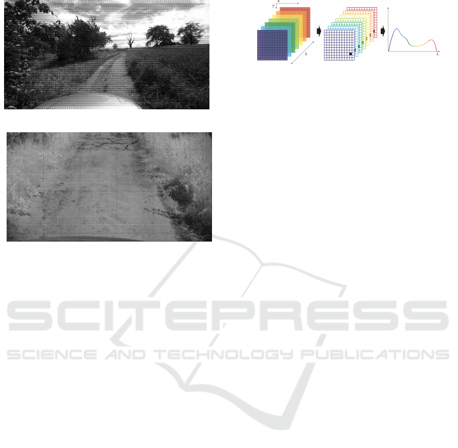
Figure 2: A schematic representation of a hypercube and an
interpolated plot of a single data point.
We define a hypercube as
H : L
x
× L
y
× L
λ
→ IR (1)
where L
x
, L
y
are the spatial domain and L
λ
the spec-
tral domain of the image.
Figure 2 shows a visual interpretation of a hyper-
cube.
The hypercube is understood as a volume, where
each point H(x, y, λ) corresponds to a spectral re-
flectance.
Derivated from the above definition a spectrum χ
at (x,y) is defined as
H(x, y) = χ, (2)
where χ ∈ IR
|L
λ
|
and |L
λ
| = n · m. The image with
only one wavelength, called a spectral band
H(z) = B
λ=z
, (3)
is defined as follows:
B
λ
: L
x
× L
y
→ IR (4)
This image contains x = (x, y) the wavelength sen-
sitivity λ for each coordinate.
4 HYPERSPECTRAL
CLASSIFICATION
Supervised learning techniques like Random Forest
need a training set, which consists of a set of sample
feature vectors coupled with a corresponding label-
ing. The labels c ∈ C are user-defined classes which
are normally represented by integer numbers. The
training and test sets are randomly composed from
our annotated dataset, which will be explained in sec-
tion 5 in more detail.
Given a set of N corresponding training pairs the
aim is to find a function γ which generalizes well
enough to new data, so accurate predictions for pre-
viously unseen data can be calculated.
γ(x) = c (5)
In this process a classifier might generate a model
which is a representation of the given problem from
which a classification can be deduced. An accurate
Hyperspectral Terrain Classification for Ground Vehicles
419

model yields better results for unseen data but highly
depends on the training data.
We have chosen to utilize a Random Forest (RF)
as a supervised classifier, because it’s fast to train and
delivers remarkable results.
Random Forests belong to the group of ensemble
classifiers and utilize a set of Decision Tree classi-
fiers to learn a robust model. Each classifier is trained
on its own subset of training data which is generated
by bagging. Bagging is a common approach where
samples are randomly drawn with replacement from
the original dataset to generate a new distribution of
the data. This prevents overfitting and yields different
patterns in the input data. The decision trees are un-
balanced binary trees. A single decision tree is com-
posed of several nodes, an unique root node, a set of
internal nodes and a set of leaves. They form an deci-
sion space with the leafs representing a class assign-
ment.
Each of its nodes is composed of a feature index
i to split on and a threshold t to split at. It classi-
fies a given feature vector x as follows. A label is di-
rectly assigned if the node is a leaf otherwise a child
node assigns the label. The left child node is used
if x[m] ≤ t otherwise the right. This recursively par-
titions the feature space beginning at the unique root
node. Building the tree is done also starting at the root
by splitting greedily. Splits are calculated by choos-
ing the best feature and the best threshold from all fea-
tures of the feature vector and a small set of thresholds
which is generated randomly. To determine the best
split, a gain is maximized. Measurement for the gain
G of a split is the weighted impurity i(x) difference
between the samples at a node and after the split
G = I(X)−
∑
i∈(l,r)
|X
i
|
|X|
I(X
i
) (6)
where X is the given set of feature vectors and X
l
/X
r
is
the set of vectors which is splitted to the left or right.
We used the gini impurity for its fast computation and
good results. Furthermore these decision trees only
use a random subset of the features for every decision
node to further increase their diversity. These deci-
sion trees, form a Random Forest, which are used to
classify the generated subsets. The result of the clas-
sification is obtained by majority voting.
In order to classify regions of an environment for
its drivability, a suitable model must be trained using
a Random Forest classifier. Since two cameras with
different wavelength sensitivities were used here, two
separate models need to be trained. However, the
recorded raw images must first be preprocessed in or-
der to filter error-prone data and then be annotated.
Since the data was taken from a vehicle driving in a
natural environment with sunlight, they are partially
under and overexposed. Therefore, these data must
first be sorted out and filtered so that a stable model
can be learned. As already mentioned in section 3, a
pre-processed image forms a hypercube with a spec-
trum of 16 or 25 spectral reflectances for each pixel
defined as χ. For training, the annotated hypercubes
are first dissected and filtered as described above. The
remaining spectra are randomly composed to test and
training data sets. As input data, a Random Forest
now receives an annotated spectrum which consists
of a 16 or 25 dimensional feature vector.
Utilizing the training set we trained a Random
Forest with ten trees for every camera. By making
use of parallelization we were able to further boost
the performance of the already fast Random Forest
classifier. To solely test the hyperspectral classifica-
tion accuracy only one spectrum χ with |L
λ
| spectral
bands has to be given to the classifier at once. This
corresponds to a per pixel classification of an image,
as further discussed in the next section.
5 EVALUATION
As far as we know, there is no publicly available data
set with hyperspectral data recorded by these special
cameras. Therefore we built our own dataset, which
will be published in the near future. We equipped
a standard car with the MQ022HG-IM-SM4X4-VIS
(VIS) and MQ022HG-IM-SM5X5-NIR (NIR) from
Ximea. The cameras are calibrated and synchronized
using a hardware trigger. We collected a total of
≈ 200GB of data driving through suburban areas,
from which we selected a subset for labeling hyper-
spectral data. As there is no labeling tool, which is
able to handle our hyperspectral data correctly, we de-
veloped our own.
The recorded and preprocessed data had then to
be annotated. This was done by hand for all images
of each dataset. During the labeling process not all
image pixels have been assigned classes. This is due
to the fact, that border areas between materials are
not unambiguously assignable. And as later results
have shown no errors arised from this constrain. The
dataset was labeled in terms of drivability. The main
classes were drivable, rough and obstacle furthermore
the class sky was introduced as an additional class, be-
cause it is an important part of our scene and defines
the border of the terrain. Furthermore it’s reflectance
is visible many places like cars. In addition a princi-
pal component analysis (PCA) was performed on this
dataset projecting it to 7 features.
Random Forests and Gaussian Naive Bayes (Chan
VISAPP 2017 - International Conference on Computer Vision Theory and Applications
420

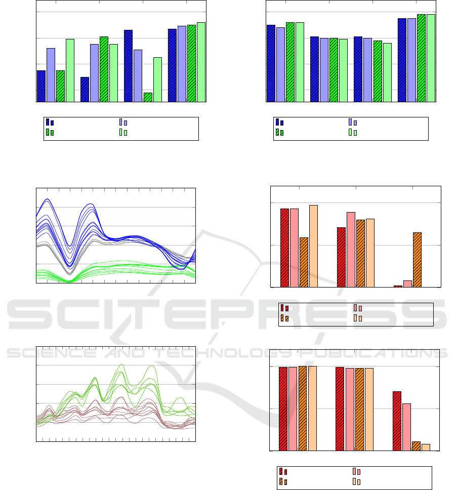
drivable rough obstacle sky
40
60
80
100
55
50
86
87
72
75
71
89
55
81
38
90
79
75
65
92
precision (raw) (%) precision (PCA) (%)
recall (raw) (%) recall (PCA) (%)
(a) Gaussian Naive Bayes.
drivable rough obstacle sky
40
60
80
100
90
81 81
95
88
80 80
95
92
80
78
98
92
79
76
98
precision (raw) (%) precision (PCA) (%)
recall (raw) (%) recall (PCA) (%)
(b) Random Forest.
Figure 3: Classification results of Gaussian Naive Bayes and Random Forest on raw and PCA data of the VIS-Camera.
468
478
490
503
514 526 541 555
569
578 592 600 611 622 642
0
0.2
0.4
0.6
0.8
1
Wavelength
Reflectance
(a) Plots of spectra captured with the VIS-Camera.
Sky (blue) street (gray) and vegetation (green).
673 674 689
714 728
740 754 767 780 791
803
822 834 844 855 865 875
884
893 909 917 924 930 939
944
0
0.2
0.4
0.6
0.8
1
Wavelength
Reflectance
(b) Plots of spectra captured with the NIR-Camera.
Street (gray) and vegetation (green).
Figure 4: Spectral plots of NIR-Camera and VIS-Camera for
different materials.
et al., 1982) have been applied to our initial training
and test datasets as well as the PCA transformed data.
It is noticeable that the Random Forest classifier
has generally produced poorer results with models
trained by using PCA data. This is consistent with the
findings of Cheriyadat (Cheriyadat and Bruce, 2003),
because of the fact that hyperspectral data is highly
correlated. The the Gaussian Naive Bayes classifier
(GNB) in contrast, produced better results with the
drivable rough obstacle
0
50
100
93
71
2
93
89
8
59
80
65
97
81
0
precision (raw) (%) precision (PCA) (%)
recall (raw) (%) recall (PCA) (%)
(a) Gaussian Naive Bayes.
drivable rough obstacle
0
50
100
99 99
70
99
98
56
100
98
11
100
98
8
precision (raw) (%) precision (PCA) (%)
recall (raw) (%) recall (PCA) (%)
(b) Random Forest.
Figure 5: Classification results of Gaussian Naive Bayes
and Random Forest on raw and PCA data of the NIR-
Camera.
PCA as indicated in figure 3. This is justified by the
fact that the GNB does not regard the data as being
correlated. However, since the spectral data are highly
correlated, this classifier does not perform well as a
consequence. The PCA implicitly introduces a decor-
relation of the data, helping the GNB.
In figure 4 several spectras of classes we recon-
Hyperspectral Terrain Classification for Ground Vehicles
421

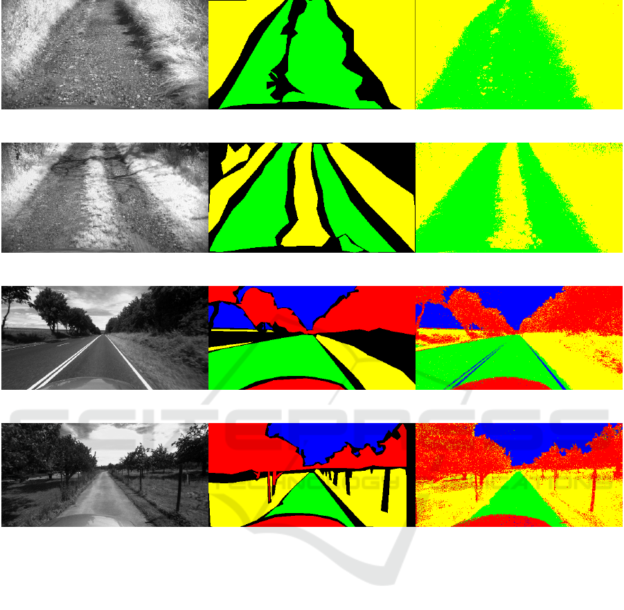
(a) Classification results of NIR data captured with the NIR-camera on a field track.
(b) Classification results of NIR data captured with the VIS-camera on a rough field track.
(c) Classification results of VIS data captured with the VIS-camera on a country road.
(d) Classification results of VIS data captured with the VIS-camera on a field track.
Figure 6: Results of our classification based on Random Forest trained with our NIR and VIS data set. The left image shows a
single spectrum, the middle is a visualisation of our annotation and the right image shows the visualized classification results.
structed are plotted, were clear differences in the
spectral reflectances of the individual classes can be
spotted. Furthermore figure 6 shows some visuali-
sations of our classification results. The classifier
was able to separate the road cleanly from rough
ground and obstacles. Figure 3 and figure 5 provide
a more detailed overview of the results. Here the ac-
curacy and precision are plotted against the respective
classes.
VIS. The VIS camera has a 5 mm lens and a fairly
wide field of view and does not only capture the ter-
rain but also the scene above. By looking at figure 3
it is striking that for all classifiers the class sky is by
far the highest. This can simply be explained by the
fact that the sky in the VIS data generally occupies a
large area. So enough records are available and the
classifier can adapt well. Furthermore, the sky has
a very characteristic radiation. Therefore it is very
easy to distinguish sky from other areas in the scenery.
The Random Forest classifier also produced notice-
able high scores for the other classes where rough
and obstacle have slightly lower scores. This might
be caused by the fact, that the classification uses only
spectral information, which can’t distinguish between
a stone wall and a stone path. Because it isn’t trained
to take context and spatial information into account.
Overall the GNB scores worse with the exception of
the raw precision for obstacles.
NIR. First it must be noted that the NIR camera, un-
like the VIS camera, has a double-telecentric 16 mm
VISAPP 2017 - International Conference on Computer Vision Theory and Applications
422

lens and is directed downwards. Therefore, it has
only recorded data from the road ahead of the vehi-
cle. This means that no data from the sky is available
and consequently can not be trained. Furthermore,
the training and test data set consists of only about
0.66% of data annotated as an obstacle. Accordingly,
the trained model is not capable of classifying obsta-
cles. This is also indicated in figure 5a where Gaus-
sian Naive Bayes is not capable of classifying obsta-
cles. The Random Forest classifier, performed best
with a precision of 70% and a recall of 56% on the
obstacle class. This suggests that 70% of the data
identified as an obstacle was actually an obstacle and
56% of all obstacles were also classified. This is quite
remarkable considering the available data.
The classes drivable and rough produced better
classification rates. This is because solid ground,
which is composed of asphalt or stones, was regarded
as being drivable. And meadows, fields, bushes and
grasses were labeled as rough. So the rough surface
consists almost exclusively of elements, which con-
tain a high proportion of chlorophyll. Elements with
chlorophyll are easily separated from elements with a
low content of chlorophyll, since chlorophyll has its
strongest absorption at about 675 nm and the absorp-
tion decreases sharply afterwards, which can be also
seen in our reconstructed spectrum in figure 4b.
6 CONCLUSION
The experiments carried out imply a Random Forest
classifier to be reliable for hyperspectral classifica-
tion in combination with the snapshot hyperspectral
cameras. The Random Forest classifier delivers de-
cent results for the NIR camera as well as for the VIS
camera. Based on the captured hyperspectral data we
were able to precisely distinguish road or drivable ar-
eas from non-drivable areas like rough or obstacles,
which could greatly enhance terrain classification per-
formance.
Furthermore, a Random Forest can be trained in a
short time in comparison to the other methods. Due
to its structure, it can be parallelized very well and ac-
celerated effectively. Another interesting result is that
the balance of the training is vital for the quality of
the classification. These promising results are a first
showcase for the capabilities of the novel sensor sys-
tem and its suitability for terrain classification, e.g. in
autonomous driving. In order to improve the pixel-
wise classification, we plan to combine it with a con-
ditional random field and to additionally add spatial
and laser data to achieve an improved classification.
ACKNOWLEDGEMENTS
This work was partially funded by Wehrtechnische
Dienststelle 41 (WTD), Koblenz, Germany.
REFERENCES
Camps-Valls, G. and Bruzzone, L. (2005). Kernel-based
methods for hyperspectral image classification. IEEE
Transactions on Geoscience and Remote Sensing,
43(6):1351–1362.
Camps-Valls, G., Gomez-Chova, L., Mu
˜
noz-Mar
´
ı, J., Vila-
Franc
´
es, J., and Calpe-Maravilla, J. (2006). Com-
posite kernels for hyperspectral image classifica-
tion. IEEE Geoscience and Remote Sensing Letters,
3(1):93–97.
Camps-Valls, G., Tuia, D., G
´
omez-Chova, L., Jim
´
enez, S.,
and Malo, J. (2011). Remote sensing image process-
ing. Synthesis Lectures on Image, Video, and Multi-
media Processing, 5(1):1–192.
Cavigelli, L., Bernath, D., Magno, M., and Benini, L.
(2016). Computationally efficient target classifica-
tion in multispectral image data with deep neural net-
works. In SPIE Security+ Defence, pages 99970L–
99970L. International Society for Optics and Photon-
ics.
Chan, T. F., Golub, G. H., and LeVeque, R. J. (1982). Up-
dating formulae and a pairwise algorithm for comput-
ing sample variances. In COMPSTAT 1982 5th Sym-
posium held at Toulouse 1982, pages 30–41. Springer.
Cheriyadat, A. and Bruce, L. M. (2003). Why princi-
pal component analysis is not an appropriate fea-
ture extraction method for hyperspectral data. In
Geoscience and Remote Sensing Symposium, 2003.
IGARSS’03. Proceedings. 2003 IEEE International,
volume 6, pages 3420–3422. IEEE.
Degraux, K., Cambareri, V., Jacques, L., Geelen, B.,
Blanch, C., and Lafruit, G. (2015). Generalized in-
painting method for hyperspectral image acquisition.
In Image Processing (ICIP), 2015 IEEE International
Conference on, pages 315–319. IEEE.
Fauvel, M., Benediktsson, J. A., Chanussot, J., and Sveins-
son, J. R. (2008). Spectral and spatial classification of
hyperspectral data using svms and morphological pro-
files. IEEE Transactions on Geoscience and Remote
Sensing, 46(11):3804–3814.
Geelen, B., Tack, N., and Lambrechts, A. (2014). A
compact snapshot multispectral imager with a mono-
lithically integrated per-pixel filter mosaic. In Spie
Moems-Mems, pages 89740L–89740L. International
Society for Optics and Photonics.
Hughes, G. (1968). On the mean accuracy of statistical pat-
tern recognizers. IEEE transactions on information
theory, 14(1):55–63.
Kriegler, F., Malila, W., Nalepka, R., and Richardson, W.
(1969). Preprocessing transformations and their ef-
fects on multispectral recognition. In Remote Sensing
of Environment, VI, volume 1, page 97.
Hyperspectral Terrain Classification for Ground Vehicles
423

Li, J., Bioucas-Dias, J. M., and Plaza, A. (2010). Semisu-
pervised hyperspectral image segmentation using
multinomial logistic regression with active learning.
IEEE Transactions on Geoscience and Remote Sens-
ing, 48(11):4085–4098.
Li, J., Bioucas-Dias, J. M., and Plaza, A. (2012). Spectral–
spatial hyperspectral image segmentation using sub-
space multinomial logistic regression and markov ran-
dom fields. IEEE Transactions on Geoscience and Re-
mote Sensing, 50(3):809–823.
Main, R., Cho, M. A., Mathieu, R., OKennedy, M. M.,
Ramoelo, A., and Koch, S. (2011). An investigation
into robust spectral indices for leaf chlorophyll esti-
mation. ISPRS Journal of Photogrammetry and Re-
mote Sensing, 66(6):751–761.
Melgani, F. and Bruzzone, L. (2004). Classification of hy-
perspectral remote sensing images with support vector
machines. IEEE Transactions on geoscience and re-
mote sensing, 42(8):1778–1790.
Plaza, A., Benediktsson, J. A., Boardman, J. W., Brazile, J.,
Bruzzone, L., Camps-Valls, G., Chanussot, J., Fauvel,
M., Gamba, P., Gualtieri, A., et al. (2009). Recent ad-
vances in techniques for hyperspectral image process-
ing. Remote sensing of environment, 113:S110–S122.
Sch
¨
olkopf, B. and Smola, A. J. (2002). Learning with ker-
nels: support vector machines, regularization, opti-
mization, and beyond. MIT press.
Tarabalka, Y., Fauvel, M., Chanussot, J., and Benediktsson,
J. A. (2010). Svm-and mrf-based method for accu-
rate classification of hyperspectral images. IEEE Geo-
science and Remote Sensing Letters, 7(4):736–740.
Tsagkatakis, G., Jayapala, M., Geelen, B., and Tsakalides,
P. (2016). Non-negative matrix completion for the en-
hancement of snap-shot mosaic multispectral imagery.
Tsagkatakis, G. and Tsakalides, P. (2015). Compressed hy-
perspectral sensing. In SPIE/IS&T Electronic Imag-
ing, pages 940307–940307. International Society for
Optics and Photonics.
Tsagkatakis, G. and Tsakalides, P. (2016). A self-similar
and sparse approach for spectral mosaic snapshot re-
covery. In 2016 IEEE International Conference on
Imaging Systems and Techniques (IST), pages 341–
345.
Tzagkarakis, G., Charle, W., and Tsakalides, P. (2016).
Data compression for snapshot mosaic hyperspectral
image sensors.
VISAPP 2017 - International Conference on Computer Vision Theory and Applications
424