Modeling Land Change using One or Two Time Points based

Calibration

A Comparison of Factors

María Teresa Camacho Olmedo

Departamento de Análisis Geográfico Regional y Geografía Física, Universidad de Granada, Spain

Keywords: Land Change Modeling, Calibration Step, Factors, Land Use and Cover Change.

Abstract: One of land change model parameters in calibration step relates to how changes over time and space are

considered in the model. A land change model can be calibrated with the state at one time point or with the

difference between two time points. The purpose is describing land use and cover (LUC) state patterns, i.e.

one time point calibration, and LUC transition patterns, i.e. two time points. For a case study in Spain we

obtained the collections of factors for two calibration periods at one time point (dates 2000 and 2006) and

the collections of factors for two calibration periods between two time points (periods 1990-2000 and 2000-

2006). Evidence likelihood is used to transform the explanatory variables into factors. The objective of this

paper is to compare these four collections of factors to show how the choice of reference maps influences

the factors and how these factors highlight the change patterns in two different calibration periods and in the

calibration of two models. As a following step the detailed results for the different factors and LUC

categories are analysed.

1 INTRODUCTION

The validity of the model and its outputs is one of

the most important challenges in land change

modeling (Paegelow and Camacho Olmedo, 2008;

Paegelow et al., 2014). Pontius and Malanson (2005)

demonstrate that output varies more as a result of the

choice of model parameters than as a result of the

choice of the model itself. One of these parameters

relates to how changes over time and space are

considered in the model, for the purpose of describing

LUC state patterns, i.e. one time point calibration, or

LUC transition patterns, i.e. two time points

calibration (Camacho Olmedo et al., 2013; Kolb et al.,

2013).

A model that is calibrated with the state at one

time point has certain advantages and disadvantages

compared to a model that is calibrated with the

difference between two time points. The first

approach does not explicitly consider the

distribution of land cover resulting from recent past

changes and instead assesses the total past changes

(Paegelow and Camacho Olmedo, 2005; Villa et al.,

2007; Conway and Wellen, 2011; Yu et al., 2011).

By contrast, the second approach evaluates the change

potential for each possible transition, where the future

potential of the space is split into specific transitions

across a finite number of LUC categories (Eastman et

al., 2005; Sangermano et al., 2010, Wang and

Mountrakis, 2011).

When calibrating the model, the patterns of change

(or change behaviour) are analyzed by a collection of

variables explaining LUC states and/or LUC

transitions. From these variables, a collection of

factors can be created with a large variety of methods

and analyses, as described in previous research into

land change modeling (Mas and Flamenco, 2011;

Pérez-Vega et al., 2012; Camacho Olmedo et al.,

2013, 2015; Kolb et al., 2013; Soares-Filho et al.,

2013; Mas et al., 2014; Osorio et al., 2015; Abuelaish

and Camacho Olmedo, 2016).

Factors can be created without references to LUC

locations, either states or transitions, using

transformation methods as natural logarithm, fuzzy,

etc. Alternatively, a collection of factors can be

made on the basis of information about LUC

locations. This is possible if methods such as

evidence likelihood are used to create the factors,

using the LUC states as the reference areas in one

time point calibration, and the LUC transitions in

two time points calibration. We chose this option

because land change models describing LUC states

or transitions must include LUC locations.

Olmedo, M.

Modeling Land Change using One or Two Time Points based Calibration - A Comparison of Factors.

DOI: 10.5220/0006384503410349

In Proceedings of the 3rd International Conference on Geographical Information Systems Theory, Applications and Management (GISTAM 2017), pages 341-349

ISBN: 978-989-758-252-3

341

Our goals are therefore to obtain and compare

factors in order to show how the choice of LUC

reference maps influences the factors, how these

factors represent the change patterns in two different

calibration periods, how these factors represent the

change patterns in the two models calibrated in

different ways, and, finally the specific behavior of

the different LUC categories and factors.

We illustrate the procedure using the TerrSet

software (Clark Labs, 2016). For a case study in

Spain, we obtained the collections of factors for two

calibration periods at one time point (dates 2000 and

2006) and the collections of factors for two

calibration periods between two time points (periods

1990-2000 and 2000-2006). Evidence likelihood is

used to transform the explanatory variables into

factors. We then compared these four collections of

factors so as to gain a better understanding of change

patterns.

2 TEST AREA AND DATA SETS

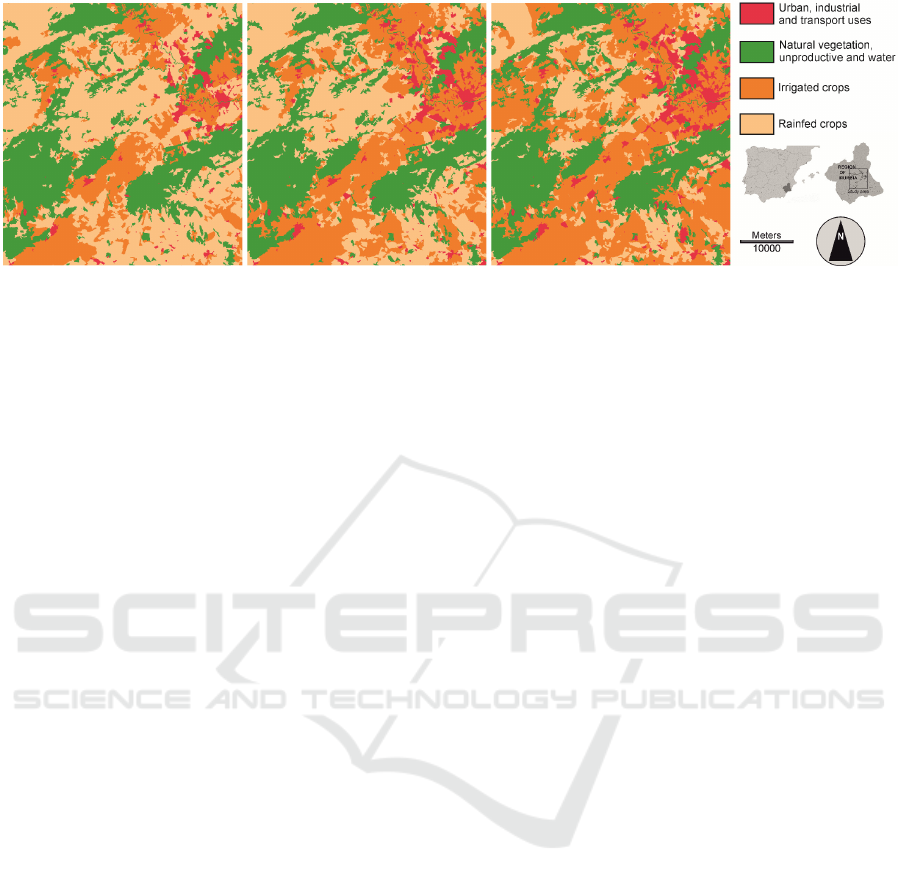
Figure 1 shows the specific study area, which covers

2,300 square kilometers in the province of Murcia

(southern Spain). The two types of calibration are

based on land use and cover data for the different

time periods and the related explanatory variables.

The maps of land use and cover (LUC) have four

categories from the Corine Land Cover

(CoORdination of INformation of the Environment,

Instituto Geográfico Nacional, Spain) dataset: urban,

industrial and transport uses; natural vegetation,

unproductive land and water; irrigated crops; rainfed

crops. In the rest of this article we refer to these

categories as urban, natural, irrigated and rainfed.

Corine maps at 1990 (t0), 2000 (t1) and 2006 (t2)

are used for model calibration. The explanatory

variables are topographic variables, protected areas,

territorial accessibility (roads diversity and quality),

distance to roads and distance to hydrographic

network (Gómez and Grindlay, 2008).

The study area has undergone profound

territorial and economic transformations in the

recent past. The most important change has been the

transition from rainfed crops to irrigated crops, due

to the development of water-related infrastructures

and the increase in the water supply (Gómez Espín

et al., 2011). Urban growth is a secondary change

driven by the development of transportation and

communication infrastructures.

3 METHODS

3.1 Obtaining Factors

Evidence likelihood is used to transform the

explanatory variables into factors. This procedure

analyzes the relative frequency of the different

categories of a given variable within the areas of

LUC states or LUC transitions. It is an efficient

means of introducing categorical variables into the

analysis, and it accepts continuous variables that

have been binned into categories.

The reference areas represented in binary maps

are therefore different for model calibration based on

one time point or two time points. For one time

point, the reference area is the most recent land use

category, i.e. the LUC state. For two time points, the

reference area is a map showing the changes that

have taken place between two points in time, i.e.

LUC transitions. This option aims to preserve the

nature of the state of the categories and the nature of

the changing categories. From now on, we refer to

areas corresponding to an LUC state or an LUC

transition as ‘reference maps’.

We obtained four reference maps for each LUC

category. In the first calibration period t0 – t1, the

reference map for one time point is a set of binary

categorical LUC maps (one for each category) at t1,

Figure1: LUC in 1990 (left), 2000 (middle) and 2006 (right) in the Murcia region in southern Spain. Source: Corine Lan

Cover.

GAMOLCS 2017 - International Workshop on Geomatic Approaches for Modelling Land Change Scenarios

342

and for two time points is a set of binary categorical

LUC maps (one for each transition) between t0 – t1.

In the second calibration period t1 – t2, the reference

map for one time point is every LUC state at t2 and

for two time points is every LUC transition between

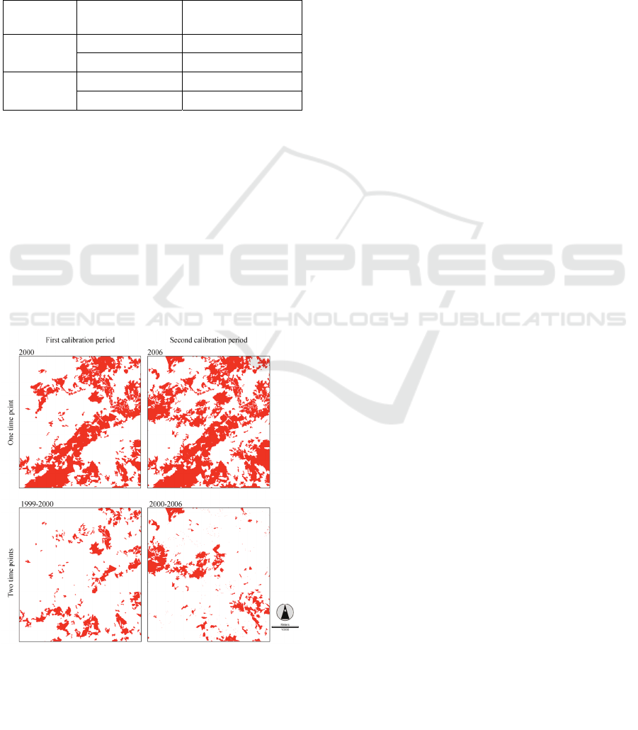
t1 – t2 (Table 1). Figure 2 shows the reference maps

for irrigated crops as an example.

Table 1: Reference maps for evidence likelihood in one

time point and two time points based calibration in both

calibration periods.

First calibration

period

Second calibration

period

One time

point

2000 (

) 2006 (

)

LUC state LUC state

Two time

points

1990 (

) – 2000 (

) 2000 (

) – 2006 (

)

LUC transitions LUC transitions

In this study we discarded the transitions

affecting small surface areas, and grouped together

the transitions involving the same final category, a

common procedure in transitions modeling. It is

important to remember therefore that we are

comparing LUC states with almost all, but not all,

the LUC transitions. In the practical application only

the following transitions are modeled:

natural/irrigated/rainfed to urban; rainfed to natural;

natural/rainfed to irrigated; natural to rainfed. By far

the most important change in the area we studied is

the transition to irrigated crops, which is followed

some way behind by urban growth.

Using these reference maps we obtained four

collections of factors for each LUC category: for one

time point and for two time points, and both of these

for two calibration periods.

3.2 Assessment Methods

The Pearson correlation, a classical method for

assessing the congruence of quantitative data, was

used for comparing factors. Instead of looking for a

causality relationship between pairs of data, the

Pearson correlation tries to establish whether there is

a relationship between them. Values range from -1

to +1. High positive/negative Pearson values

indicate a direct/indirect relationship between two

data. Low positive/negative values indicate a lack of

relationship.

The Pearson correlation was calculated between

all pairs of factors for the one and two time points

based models and for the two calibration periods.

Factors are quantitative data from 0.0 to 1.0. The

higher the Pearson coefficient, the stronger the

correlation of factors. We consider values of over

0.8 to be very strong correlations.

4 RESULTS AND DISCUSSION

4.1 Collection of Factors

For one time point and for two time points, and for

each of the two calibration periods, the collections of

factors were obtained for each LUC category. As an

example, Figures 3 and 4 show the collection of

factors derived from the elevation variable and from

the slope variable in the reference maps for irrigated

crops.

4.2 Comparison of Four Collections of

Factors

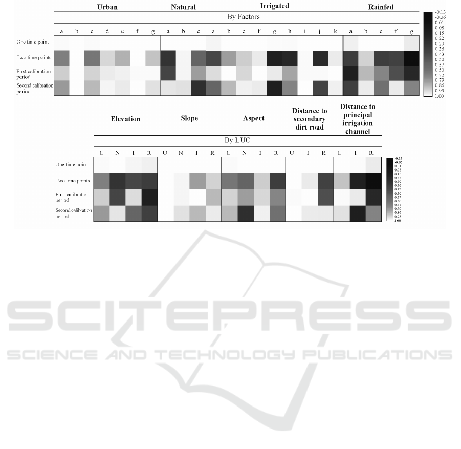
In Figure 5, the Pearson correlation values for every

pair of factors (each square corresponds to one

comparison) is showed. Each cross tabulation matrix

is composed of one column per factor grouped by

LUC category (above) or per LUC category grouped

by factors (below) and by four rows: One time point

based model (first and second calibration period),

Two time points based model (first and second

calibration period), First calibration period (one and

two time points based model), Second calibration

period (one and two time points based model).

In Figure 5 (above), the collections of factors for

the urban category are all very similar. This means

Figure 2: Reference maps for evidence likelihood of the

LUC state of irrigated crops in 2000 and in 2006 (above)

and of the LUC transition to irrigated crops over the

periods 1990-2000 and 2000-2006 (below).

Modeling Land Change using One or Two Time Points based Calibration - A Comparison of Factors

343

that transitions patterns to this category are very

close to the state pattern for this category in both

calibration periods. The only exceptions are the

elevation and aspect factors. As an example, if we

focus on the Pearson correlation values for elevation

factors related to the urban category, we can see that

for 2000 and 2006 the situations are almost identical

(first row); the transitions between 1990-2000 and

2000-2006 are not so close (second row); the state in

2000 is very similar to the transitions over the period

1990-2000 (third row); and the state in 2006 is less

similar to the transitions that took place over the

period 2000-2006 (fourth row).

The factors for the natural vegetation,

unproductive and water category and the factors for

irrigated crops vary more sharply: transition patterns

in the first calibration period are not similar to those

in the second. Transitions are not very close to the

state pattern in either period. With respect to

irrigated crops, in the second calibration period the

transitions patterns are quite different from the state

pattern. This is due to elevation, distance to a main

irrigation channel and distance to a network of

ditches. Finally, for the collection of factors for

rainfed crops, a high dissimilarity is present in

transition patterns for both calibration periods and

with respect to the state pattern, particularly in the

first calibration period. However, it is also important

to emphasize that the state patterns are stable for all

categories (first row in Figure 5, above, one time

point based model).

In brief, if we compare the two calibration

methods, there is a medium to high linear

relationship between LUC transitions and LUC

states, which is higher in the first calibration period

in all the categories except for one. Looking at each

category, the urban patterns are very stable while at

the opposite extreme, the patterns for rainfed crops

show high variation. The situation also varies a great

deal in the natural category and in irrigated crops:

the transition patterns are not very stable and are not

very similar to the state pattern.

In Figure 5 (below), the Pearson values are

grouped by factors. Only factors common to at least

two LUC categories are shown. A quick overview

confirms that the state patterns are stable for all

categories (first row, one time point based model).

Aspect is the factor with the highest values in both

calibration periods and both models, followed by

distance to secondary road, except in the rainfed

crops category. Elevation and aspect seem to be the

most sensitive factors. They show widely varying

behavior, with high, medium and low Pearson

values, which means that transition patterns and

state patterns are not regular with respect to these

variables. With regards to distance to main irrigation

channel, the transition patterns for irrigated crops are

not regular, although the most irregular are those for

Figure 3: Irrigated crops and elevation. Evidence

likelihood of the LUC state for irrigated crops in 2000 an

2006 derived from the elevation variable (above) and o

the LUC transition to irrigated crops over the periods

1990-2000 and 2000-2006 derived from the elevatio

variable (below).

Figure 4: Irrigated crops and slope. Evidence likelihood o

the LUC state for irrigated crops in 2000 and 2006 derive

from the slope variable (above) and of the LUC transitio

to irrigated crops over the periods 1990-2000 and 2000-

2006 derived from the slope variable (below).

GAMOLCS 2017 - International Workshop on Geomatic Approaches for Modelling Land Change Scenarios

344

rainfed crops. In brief, when looking at the different

factors, the homogeneity or heterogeneity of LUC

locations can lead to widely varying behavior.

Previous researchers observed a relationship

between environmental and accessibility factors and

the initial conditions in which LUC changes are

carried out (Lambin et al., 2001; Yu et al., 2011

Osorio et al., 2015).

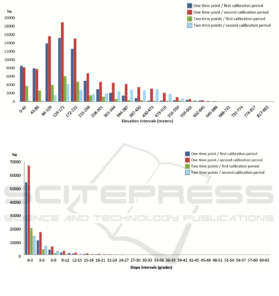
For a better understanding of these patterns, we

focused on the collection of factors for irrigated

crops. Figures 6 and 7 present the histograms (ha)

for the LUC state for irrigated crops in 2000 and

2006 and for the LUC transition to irrigated crops

over the periods 1990-2000 and 2000-2006, by

elevation intervals and by slope intervals.

If we compare these two variables, we can

conclude that irrigated crops behave in a more

homogenous manner with respect to slope (only

some slope intervals are affected) than to elevation,

which explains the different Pearson values

commented above. Figure 6 shows that irrigated

crops were located at lower elevations in the first

calibration period, 1990-2000, and that the new

irrigated fields planted from 2000 to 2006, went up

to higher elevations, in other words, transitions

occurred at different altitudes. However, we do not

know if this is a general dynamic or if it is due to the

particular behavior of one of the LUC origin

categories (natural or rainfed). We must remember

that, in this study, we grouped some transitions

(natural/irrigated/rainfed to urban; natural/rainfed to

irrigated) together. Although this is a common

procedure in modeling, it does not allow us to

distinguish between the categories that have been

grouped together.

Figures 6 and 7 show absolute surface area

values (ha), which means that comments must also

be relativized with respect to the surface areas of the

reference maps. We assume that an LUC state or an

LUC transition with a larger area offers more robust

statistical representativeness. This means that the

factors that are created and their patterns should be

more stable. On the other hand, if the surface areas

of the reference maps of LUC states and of LUC

transitions are similar in size, the patterns should

also be more similar, because the LUC transitions

are included in the LUC state for the same

calibration period.

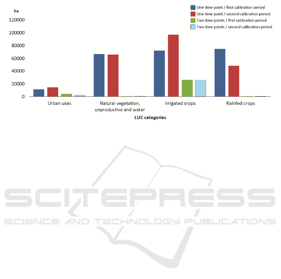
Figure 8 presents the surface area (ha) for the

reference maps for all the LUC categories. As

commented earlier, we decided not to model very

small transitions or grouped heterogeneous

transitions. For the natural category and the rainfed

category, the surface areas of LUC states and LUC

Figure 5: Representation of Pearson correlation values for each pair of factors (each square corresponds to one comparison).

Each cross tabulation matrix is composed of one column per factor grouped by LUC (above) and per LUC grouped by

factors (below), and of four rows: One time point based model (first and second calibration period), two time points base

model (first and second calibration period), first calibration period (one and two time points based model), secon

calibration period (one and two time points based model). Factors legend (above): elevation (a), slope (b), aspect (c),

accessibility to main road (d), accessibility to human settlements (e), distance to secondary road (f), distance to mai

irrigation channel (g), distance to secondary irrigation channels (h), distance to network of rivers and streams (i), distance to

network of ditches (j), distance to water catchments (k). LUC legend (below): urban (U), natural (N), irrigated (I) rainfed (R).

Modeling Land Change using One or Two Time Points based Calibration - A Comparison of Factors

345

transitions vary greatly and may therefore show a

different pattern in the extracted factors. Besides,

LUC transitions to these categories in both

calibration periods affect only a small proportion of

the study area (<900 ha in the natural category, <400

ha in the rainfed crops category). In fact, LUC

transitions to the natural category correspond to less

than 2% of the natural LUC state, and LUC

transitions to the rainfed category correspond to less

than 1% of the rainfed LUC state. Therefore,

modeling LUC transitions may not be statistically

representative.

For irrigated crops, even if the surface areas of

LUC state and LUC transitions vary greatly, they

still correspond to 26,386 and 26,026 ha or 36% and

27% of the LUC state for irrigated crops in the two

calibration periods respectively. The total surface

area covered by urban areas is lower than the other

categories, but LUC transitions, with 4,513 and

2,969 ha in the two calibration periods, correspond

to 38% and 20% of urban LUC states respectively.

This means that modeling LUC transitions for these

categories can be statistically representative.

Valuable additional information can be obtained

by assessing the coincidence between the reference

Figure 6: Histograms (ha) for the LUC state for irrigated crops in 2000 and 2006 and for the LUC transition to irrigate

crops over the periods 1990-2000 and 2000-2006, by elevation intervals.

Figure 7: Histograms (ha) for the LUC state for irrigated crops in 2000 and 2006 and for the LUC transition to irrigate

crops over the periods 1990-2000 and 2000-2006, by slope intervals.

GAMOLCS 2017 - International Workshop on Geomatic Approaches for Modelling Land Change Scenarios

346

maps for the two calibration periods. As commented

in section 3.1., there is no coincidence between the

areas of the reference maps in the two time points

based model. In the one time point based model, the

coincidence between the area in the first calibration

period with respect to the area in the second

calibration period is 100% for urban areas, 97.71%

for the natural category, 97.51% for irrigated crops

and 63.86% for rainfed crops. However, the

coincidence between the areas in the second

calibration period with respect to the area in the first

calibration period is 79.97% for urban areas, 98.66%

for the natural category, 73.20% for irrigated crops

and 98.84% for rainfed crops.

This study can be continued by comparing and

assessing the soft-classified maps obtained by the

different calibration based models. Camacho

Olmedo et al. (2013) compared suitability maps (one

time point based model) and transition potential

maps (two time point based model) in one

calibration period. The applied assessment method

showed moderate-to-high correlation values between

them, inchange-prone areas, for all categories except

one. They assessed the predictive ability of soft-

classified maps with respect to real maps, and

confirmed that a two time points based model

outperformed a one time point based model in the

case of modeling urban growth because the

transition potential map for urban growth captured

urban change more accurately than the suitability

map did, while the opposite was true for the other

categories.

Current research into land change models tends

to range from pattern-based models, which are

calibrated on the basis of trends observed in the past,

to models that try to simulate general processes of

change by integrating expert knowledge (NRC,

2013; Mas et al., 2014; Osorio et al., 2015).

5 CONCLUSIONS

A land change model can be calibrated with the state

at one time point or with the difference between two

time points. These approaches therefore involve

modeling either LUC states or LUC transitions. The

first approach implicitly includes all past changes,

while the second considers past changes that

occurred during a recent period. The calibration of

land change models by one time point or two time

points, i.e. states or transitions, gives different

results. The choice of reference maps affects the

similarity or dissimilarity of factors.

Factors obtained from the LUC state (one time

point based model) in two calibration periods show a

high linear relationship. The state pattern is therefore

stable. The one time point based calibration model

could therefore be accurate at modeling categories in

which transitions affect a proportionally small area

and also when patterns of change vary in recent

periods. This “total past trend” based calibration is

more likely to capture historic patterns of change

and simulations over longer time.

Factors obtained from LUC transitions (two time

points based model) in two calibration periods show

highly varied values, from non-linear to highly

linear relationships between them. Modeling LUC

transitions can be statistically representative when

they correspond to a proportionally larger area and

when patterns of change are maintained over two

Figure 8: Surface area (ha) of reference maps for the different LUC categories.

Modeling Land Change using One or Two Time Points based Calibration - A Comparison of Factors

347

successive periods. This “two past trend” based

calibration is more likely to capture recent patterns

of change and simulations over shorter periods.

A multi-temporal approach, integrating data

about more than two training dates, could resolve

potential errors resulting from only considering two

past dates or by considering the total past, and would

be more appropriate for creating forecasting

scenarios. However, a choice must be made between

using states or transitional data in the calibration of

the models. Depending on multiple parameters,

including form and intensity of dynamics, the two

approaches may be complementary.

ACKNOWLEDGEMENTS

This work was supported by the BIA2013-43462-P

project funded by the Spanish Ministry of Economy

and Competitiveness and by the Regional European

Fund FEDER.

REFERENCES

Abuelaish, B., Camacho Olmedo, M.T., 2016. Scenario of

land use and land cover change in the Gaza Strip using

remote sensing and GIS models. Arab J Geosci (2016)

9:274.

Camacho Olmedo M.T., Paegelow M., Mas, J.F., 2013.

Interest in intermediate soft-classified maps in land

change model validation: suitability versus transition

potential. International Journal of Geographical

Information Science 27 (12): 2343–2361.

Camacho Olmedo, M.T., Pontius R.G. Jr., Paegelow M.,

Mas, J.F., 2015. Comparison of simulation models in

terms of quantity and allocation of land change.

Environmental Modelling & Software, 69 (2015):

214–221.

Clark Labs, 2016. Available from: http://www.clarklabs.org/.

Conway T.M., Wellen, C.C., 2011. Not developed yet?

Alternative ways to include locations without changes

in land use change models. International Journal of

Geographical Information Science, 25 (10): 1613–

1631.

NRC, 2013. Advancing Land Change Modeling:

Opportunities and Research Requirements. Committee

on Needs and Research Requirements for Land

Change, Modeling; Geographical Sciences

Committee; Board on Earth Sciences, and Resources;

Division on Earth and Life Studies, National Research

Council, Washington, USA.

Eastman, J.R., Solorzano, L.A., Van Fossen M.E., 2005.

Transition potential modeling for land cover change.

In: Maguire, D.J., Batty, M., Goodchild, M.F. (eds.)

GIS, spatial analysis, and modeling. Redland, CA:

ESRI, pp 357–385.

Gómez Espín, J.M., López Fernández, J.A., Montaner

Salas, M.E., (eds.) 2011. Modernización de regadíos:

Sostenibilidad social y económica. La singularidad de

los regadíos del Trasvase Tajo-Segura. Colección

Usos del agua en el territorio. Universidad de Murcia.

Spain.

Gómez, J.L., Grindlay, A. (eds.) 2008. Agua, Ingeniería y

Territorio: La transformación de la cuenca del río

Segura por la IngenieríaHidráulica. Ministerio de

Medio Ambiente, Medio Rural y Marino.

Confederación Hidrográfica del Segura. Spain.

Kolb, M., Mas, J.F., Galicia, L., 2013. Evaluating drivers

of land-use change and transition potential models in a

complex lanscape in Southern Mexico. International

Journal of Geographical Information Science

27(9):1804–1827.

Lambin, E. et al., 2001. The causes of land-use and land

cover change: moving beyond the myths. Global

Environmental Change 11(4):261–269.

Mas, J.F., Flamenco-Sandoval, A., 2011. Modelación de

los cambios de coberturas/uso del suelo en una región

tropical de México. GeoTrópico, 5(1):1–24.

Mas, J.F., Kolb, M, Paegelow, M., Camacho Olmedo,

M.T., Houet, T., 2014. Inductive pattern-based land

use / cover change models: A comparison of four

software packages. Environmental Modelling &

Software, 51(2014): 94–111.

Osorio, L.P., Mas, J.F., Guerra, F., Maass, M., 2015.

Análisis y modelación de los procesos de

deforestación: un caso de estudio en la cuenca del río

Coyuquilla, Guerrero, México. Investigaciones

Geográficas, Boletín, núm. 88:60–74.

Paegelow, M., Camacho Olmedo, M.T., 2005. Possibilities

and limits of prospective GIS land cover modeling – a

compared case study: Garrotxes (France) and Alta

Alpujarra Granadina (Spain). International Journal of

Geographical Information Science, 19 (6):697–722.

Paegelow M., Camacho Olmedo, M.T., (eds.) 2008.

Modelling environmental dynamics. Advances in

geomatics solutions. Berlin: Springer-Verlag.

Paegelow M., Camacho Olmedo, M.T., Mas, J.F., Houet.

T., 2014. Benchmarking of LUCC modelling tools by

various validation techniques and error analysis.

Cybergeo, document 701, mis en ligne le 22 décembre

2014.

Pérez-Vega, A., Mas, J.F., Ligmann-Zielinska, A., 2012.

Comparing two approaches to land use/cover change

modeling and their implications for the assessment of

biodiversity loss in a deciduous tropical forest.

Environmental Modelling & Software 29 (1):11–23.

Pontius, R.G.,Jr., Malanson, J., 2005. Comparison of the

structure and accuracy of two land change models.

International Journal of Geographical Information

Science 19:243–265.

Sangermano, F., Eastman, J.R., Zhu, H. 2010. Similarity

weighted instance based learning for the generation of

transition potentials in land change modeling.

Transactions in GIS 14(5):569–580.

Soares-Filho, B., Rodrigues, H., Follador, M., 2013. A

hybrid analytical-heuristic method for calibrating land-

GAMOLCS 2017 - International Workshop on Geomatic Approaches for Modelling Land Change Scenarios

348

use change models. Environmental Modelling &

Software 43(2013):80–87.

Villa, N., et al., 2007. Various approaches for predicting

land cover in Mediterranean mountains.

Communication in Statistics 36(1):73–86.

Wang, J., Mountrakis, G., 2011. Developing a multi-

network urbanization model: a case study of urban

growth in Denver, Colorado. International Journal of

Geographical Information Science 25(2):229–253.

Yu, J., et al., 2011. Cellular automata-based spatial multi-

criteria land suitability simulation for irrigated

agriculture. International Journal of Geographical

Information Science 25(1):131–148.

Modeling Land Change using One or Two Time Points based Calibration - A Comparison of Factors

349