Optimal 3D Kinematic Analysis for Human Lower Limb Rehabilitation

Hachmia Faqihi

, Maarouf Saad

, Khalid Benjelloun

, Mohammed Benbrahim

and M. Nabil Kabbaj

LAII, Ecole Mohammadia d’Ingnieurs, Mohammed V University, Rabat, Morocco

Ecole de Technologie Suprieure, Montreal, Canada

LISTA, Faculty of Sciences, University of Fez, Morocco

Keywords:

Robotics, Rehabilitation, Inverse Kinematics, Human Leg, Trajectory Generation, Optimization, Minimum

Jerk.

Abstract:

The majority of the kinematics analysis carried out on the human body are usually available only for use in

the sagittal plane. Limited studies were interested in this analysis in all three planes (sagittal, transverse, and

frontal) where motions of all joints occur.

The aim of this paper is to develop a new optimal kinematic analysis of human lower limbs in three-

dimensional space for a rehabilitation end. The proposed approach is focused on optimizing the manipulability

and the human performance of the human leg, as being a physiologically constrained three-link arm. The ob-

tained forward kinematic model leads to deﬁne the feasible workspace of the human leg in the considered

conﬁguration. Using an effective optimization-based human performance measure that incorporates a new

objective function of musculoskeletal discomfort, the optimal inverse kinematic (IK) model is obtained.

1 INTRODUCTION

Nowadays several neurologic injuries such as neuro-

muscular diseases, spinal cord injury cerebellar dis-

orders, stroke, or impaired functions of the member

musculature lead to the joint disorders. Indeed, the

lower limb is usually including chronic pain, atypical

gait patterns, reduced range of motion (ROM), weak

strength, and increased joint stiffness, as well as se-

vere functional limitations, and thereby reducing pa-

tient’s quality of life.

To remedy these problems, we use the rehabili-

tation process, based on physical therapy to restore

patient’s strength, mobility and ﬁtness. Traditionally,

limb physical therapy sessions were carried out man-

ually with assistance of therapists. However, the poor

performances in terms of duration, strength and task

orientation of the training, and the inconsistency in

therapy sessions from one session to another have

been noted, as principles issues, to encouraged many

researchers to require the robotic, where a good re-

peatability, and a precisely controllable assistance,

providing quantitative measures of the subject’s per-

formance and reducing the required labor of physi-

cal therapists are carried out. Therefore, the use of

robotics in this context needs to take into account the

different biomedical constraints imposed in the study

of this system (H. Faqihi and Kabbaj, 2016).

Generally, robotic is largely used in many applica-

tions such as medical, physical and industrial, where

high accuracy, repeatability, and stability of the op-

erations are required. For different robotic studies,

the developpement of control laws is commonly exe-

cuted in joint space. Howerver, the motion planning

is given in the task space, especially when it comes to

real applications as rehabilitation, where the desired

input is usually the end effector position in task space.

Hence the necessity to resorting to the Inverse Kine-

matic (IK) task to ﬁnd a conﬁguration at which the

end-effector of the robot reaches a given point in the

task space.

Several researches have been provided to derive

the IK problem, especially for redundant articulated

robotic arm, such as a parts of human body, where the

complexity is enhanced with the increased Degrees

Of Freedom (DOF). Thereby, solving the IK problem

is quite a challenging task, where its complexity lies

in the robots geometry and nonlinear relation between

cartesian and joint space.

The most popular IK methods developed in

the literature are algebraical, geometrical methods

(W. M. Spong and Vidyasagar, 2006), and the analyt-

Faqihi, H., Saad, M., Benjelloun, K., Benbrahim, M. and Kabbaj, M.

Optimal 3D Kinematic Analysis for Human Lower Limb Rehabilitation.

DOI: 10.5220/0006477701770185

In Proceedings of the 14th International Conference on Informatics in Control, Automation and Robotics (ICINCO 2017) - Volume 1, pages 177-185

ISBN: 978-989-758-263-9

177

ical methods (A. Ochsner, 2014), using the pose (po-

sition and orientation) as a given goal, (V. Kumar and

Shome, 2015), (S. Tejomurtula, 1999), (J.M.Porta,

2005). They are usually designed for a very spe-

ciﬁc task, and remain very limited for the higher DOF

robots. They do not guarantee closed form solutions,

and they are entirely sensible to the starting point and

singular conﬁguration problem.

Taking into account the dynamic of motion, the

Jacobians method can also be used to resolve the IK

problem, but it has been pointed out that it does not

provide all credible solutions. Additionally, these

traditional solution methods may have a prohibitive

computational cost because of the high complexity of

the geometric structure of the robotic manipulators.

To summarize, the application of the classical IK

methods for the human body, besides its complexity,

remains just viable mathematically, do not take into

account the physiological feasibility and bioﬁdelity of

human posture, and suffer from numerical problems

(K.Abdel-Malek, 2004) .

Optimization based approaches can be suitable ways

to overcome the above mentionned problems. It refers

to predict the realistic posture of human limb in its

feasible workspace. As any optimization problem, for

the posture prediction problem, the joint angles of the

human leg are considered as the design variables, the

constraints are considered according to physiological

feasibility and motion precision, and for the objective

function, the human performance measures are used.

There are many forms used in the literature to de-

ﬁne the human performance measure, such as phys-

ical fatigue deﬁned as reduction of physical capac-

ity. It is mainly the result of three reasons: magni-

tude of the external load, duration and frequency of

the external load, and vibration (Chen, 0004). How-

ever, for the movements required low speed such as

rehabilitation exercises, the physical fatigue is not so

signiﬁcant. Indeed, the required movements can lead

to some human discomfort (K.Abdel-Malek, 2004),

where its evaluation may vary from person to person,

such as potential energy (Z. Mi, 2009), torque joints,

muscle fatigue, or perturbation from a neutral position

(W. M. Spong and Vidyasagar, 2006).

This study seeks to introduce a general

optimization-based formulation for posture pre-

diction of human lower limb exclusively in all

sagittal, transverse, and frontal planes with seven

degrees of freedom. Refering to the published

studies, the proposed kinematic analysis is the

ﬁrst one developed in 3D plane. A new objective

function incorporating three factors that contribute to

musculoskeletal discomfort is developed as human

performance measure.

To better illustrate these aspects, the remainder of

the paper is organized as follows: In section II, the

human leg modeling will be presented. The forward

kinematics has been developed in the three planes

where motions of the human lower limb occur with

seven degrees of freedom. According to that, in sec-

tion III, the feasible workspace have been established.

In section IV, the new optimal posture prediction has

been described and thereby applied on the human

lower limb for the provided motion conﬁguration. To

check the effectiveness of the proposed approach, in

section V, a simulation model has been developed us-

ing Matlab package. To sum up, the results of the

study are outlined in section VI.

1.1 Human Lower Limb Description

The human body is a complex system, its biomechani-

cal modeling represents a simpliﬁcation of its real op-

erating. The introduction of assumptions is necessary

in this order, which are selected according to the de-

sired performances.

The model adopted for the lower limb represents a

system of articulated links connected by joints, based

on three segments to model its anatomical structure:

thigh, shank and foot considered as the length be-

tween ankle and metatarsal.

The connection of all three segments is ensured

naturally by ligaments and muscles, and should be

kinematically redundant to ensure bioﬁdelity of the

human leg motion (S. Tejomurtula, 2005).

For a static analysis, the human leg is modeled

by a kinematic chain of rigid bodies, interconnected

by kinematic joints, which can be either simple or

complex according to required physiological behav-

ior, and thus the degree of freedom associated with

the possible joints. The principal joints are hip, knee,

and ankle (H. Faqihi and Kabbaj, 2016).

According to the special rehabilitation use, we

are interested in this study, to the human leg

motion provided in three planes of the space,

where the motion of the human leg is provided

for sevens degree-of-freedom, deﬁned as: 3 DOF

hip (extension-ﬂexion degree-of-freedom, abduction-

adduction degree-of-freedom, and inversion-eversion

degree-of-freedom), 1 DOF knee (extension-ﬂexion

degree-of-freedom), 3 DOF ankle (extension-ﬂexion

degree-of-freedom, abduction-adduction degree-of-

freedom, and inversion-eversion degree-of-freedom),

as depicted in ﬁgure 1.

ICINCO 2017 - 14th International Conference on Informatics in Control, Automation and Robotics

178

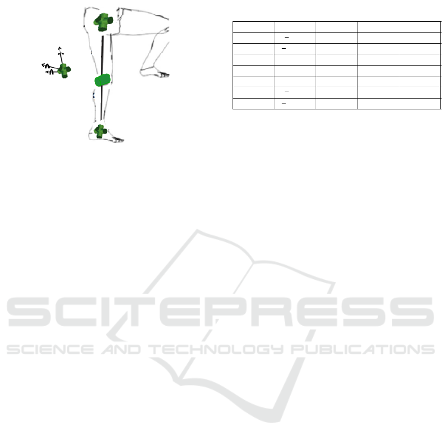
Figure 1: Coordinate systems on 7 DOF of the human leg.

1.2 Anthropometric Parameters

The modeling of body segments must take into ac-

count some anthropometric parameters.

In order to customize the model, accurate mea-

surements of the anthropometric parameters are re-

quired and can be obtained from statistical tables pro-

posed in (S. Tejomurtula, 2005). It refers to adopt a

proportional anthropometric model, based on statisti-

cal regression equations to estimate these segmental

inertial parameters (PIS).

For this study, physical length segments will be

used. They can be computed using total body height

(H).

1.3 Range of Motion

Due to the biomechanical constraints of human body

motion, the bounds of the joint variables are ﬁxed,

which deﬁne the Range of Motion (ROM).

Deﬁning ROM of the human lower limb model, is

not limited to the designed mechanical structure, but

also to the human physiological factors, such as the

age, body build, gender, health condition (D.B. Chaf-

ﬁn, 1992). Generally, the ROM of human legs, based

on a previous study by (C.S. Hernandez and Rodr-

guez, 2011) is given in the table I.

1.4 Comfort Zone

To ensure the comfort motion of the human body,

each joint variable can be deﬁned by its comfort zone,

which must belong to the range of motion (ROM) of

the associated joint variable.

Referring to the literature, the comfort zone repre-

sents 35% of the range of motion (ROM). The center

of the comfort zone, q

, is calculated by the following

expression (S. Glowinski, 2016):

Table 1: DH human leg parameters for 5dof.

Joint(i) α

0 0 q

3 0 a

0 q

4 0 a

0 q

5 0 a

0 q

0 0 q

= 0.5(q

icz

+ q

icz

) + q

(1)

where q

icz

, and q

icz

are respectively, the upper and

lower angles of the comfort zone, for the i

joint vari-

able associated. q

is the home position angle of the

joint variable. Generally, the home position an-

gle can differ from tested tasks (standing, recumbent,

seating,...).

2 FORWARD KINEMATIC

ANALYSIS

The forward kinematic (FK) model in n plane, can

determine the pose of the end-effector (x

, j = 1...n),

from given joint variables (q

,i = 1 .. .DOF). It is a

necessary step in the kinematic anlysis process.

= f (q

) (2)

For the rigid bodies robotic systems, several methods

can be used to resolve this problem.

Despite of the human body complexity, for all

practical purposes, it has been shown that approxi-

mated modeling of gross human motion, in order to

ensure human motion simulation, ergonomic analy-

sis, or rehabilitation process, can be achieved using

homogenous transformation matrices method, and the

Denavit Hartenberg (DH) representation, based on

appropriate kinematic coordinates.

Indeed, the DH method provides an adequate, and

systematic method for embedding the local coordi-

nate systems for each link.

The forward kinematic human leg model is devel-

opped from the DH parameters (Dombre and Khalil,

2007) where each degree-of-freedom can be modelled

as a revolute joints. The DH parameters are depicted

in table 1, from the deﬁned kinematic coordinates.

From the provided D-H parameters, the forward

kinematic model can be computed using the trans-

fomation matrix, given in relation 3. Generally, the

transformation matrix is the relationship expression

between two consecutive frames i−1 and i, which de-

pends on the described parameters (q

,α

) given

Optimal 3D Kinematic Analysis for Human Lower Limb Rehabilitation

179

in the Table II.

i−1







−sq

cα

sα

−cq

sα

0 sα

cα

0 0 0 1







(3)

The global transformation matrix for seven DOF can

be expressed by:

(4)

From

the forward kinematic model is given by

the following equation:













1234

+ a

123

+ a

1234

− a

1234

+ a

123

+ a

1234

+ a

1234

−a

− a

234

− a

234

− a

234





(5)

where: c

1234

= cos(q

+ q

), s

1234

sin(q

), c

123

= cos(q

), s

123

sin(q

+ q

), c

= cos(q

+ q

), s

= sin(q

), c

= cos(q

), s

= sin(q

), and s

= sin(q

In terms of velocitiy and acceleration, the forward

kinematic is given by:

˙x

= J ˙q

, ¨x

= J ¨q

J ˙q

(6)

where ˙x

, ¨x

, represent respectively the end-effector

velocity, the end-effector acceleration in task space,

J and

J, represent the jaccobian matrix of the system

and its deerivative. Finally, and ˙q

and ¨q

represent

respectively the end-effector velocity and acceleration

in joint space.

2.1 Feasible Workspace

In order to analyze the feasible workspace associated

to the human lower limb, where we plot the differ-

ent possible positions of foot which can be achieved,

the direct kinematic model f (q

) is used. Thus, the

workspace can be deﬁned as the set of all the possible

positions in the task space according to the ROM, as

following:

= {q

∈ ROM/

∑

= f (q

)} (7)

Using the appropriate forward kinematic model given

in equation 5, and the ROM described in the table I,

the feasible workspace can be plotted for the motion

provided according to the used conﬁguration.

3 PROPOSED OPTIMIZATION

APPROACH

3.1 Problem Formulation

The optimal posture prediction is considered to be a

constrained optimization problem (CO), using a con-

straint to ﬁnd a realistic conﬁguration.

Generally, the CO problem can have equality and/or

inequality constraints according to the described

problem, and the objective function, which requires

some assumptions according to the continuity and dif-

ferentiability. In that fact, in the following the opti-

mization problem model are described:

3.1.1 Design Variables

The design variables represent in this case, the joint

variables q

, i = 1...DOF, following the used conﬁg-

uration.

3.1.2 Constraints

The ﬁrst constraints consider the difference between

the current end-effector position, velocity, and accel-

eration, and the given target position, velocity and ac-

celeration respectively in cartesian space, as follow-

ing:

||x

computed

) − x

desired

)|| ≤ ε

|| ˙x

computed

) − ˙x

desired

)|| ≤ ε

(8)

|| ¨x

computed

) − ¨x

desired

)|| ≤ ε

(9)

where ||.|| deﬁne the euclidean norm. The end-

effector position x

computed

hits a predetermined target

point x

desired

in cartesian space, within a speciﬁed tol-

erance ε

a small positive number that approximates

zero, similarly to end-effector velocity and accelera-

tion.

It should be noted that, determining the end-

effector position, velocity and acceleration are en-

sured using the forward kinematic model (equations

5, 6 and 7).

On the other hand, each joint variable is con-

strained to lower and upper limits, represented by q

and q

, respectively. These limits ensure that the hu-

man posture does not assume an unrealistic position

to achieve the target point.

To more rigorous bioﬁdelity end, we can choose

that each joint variable is constrained to lie between

upper and lower angles of the comfort zone, designed

by q

icz

and q

icz

respectively.

icz

≤ q

icz

(10)

ICINCO 2017 - 14th International Conference on Informatics in Control, Automation and Robotics

180

Finaly, the constraints in term of velocity and accel-

eration limits are used, as following.

˙q

≤ ˙q

(11)

¨q

≤ ¨q

(12)

where ˙q

and ¨q

are the lower limit of velocity and ac-

celeration, ˙q

, and ¨q

are the upper limits of velocity

and acceleration respectively. These limits are ﬁxed

according to biomedical studies, where the physiolog-

ical and health state of patient are taken into account.

3.1.3 Cost Function

As described previously, the posture prediction re-

quires a human performance measure, where its rig-

orous choice ensures the optimal realistic posture.

To this end, the modeling musculoskeletal discomfort

is used as human performance measure, which can be

somewhat ambiguous, as it is a subjective quantity,

thus its evaluation may vary from one person to an-

other (K.Abdel-Malek, 2004).

According to the last described researches

(K.Abdel-Malek, 2004; Z. Mi, 2009), in this order,

different forms of human performance measures have

been adopted, but it often results in postures with

joints extended to their limits, and thus to some un-

comfortable positions.

As remedy, we can add factors associated with

moving while joint variables are near their respective

limits in terms of position, velocity and acceleration.

In this respect, it is possible to incorporate different

factors that contribute to discomfort. The ﬁrst fac-

tor, is referred to the tendency to move different seg-

ments of the body sequentially. The second factor, is

referred to the tendency to gravitate to a reasonably

comfortable position. Finally, the discomfort associ-

ated to the motion while joints are near their ROM in

term of position, velocity and acceleration, expresses

the third factor.

According to the previous studies, the proposed

objective function is similar to that adopted by

(J.Yang, 2004) applied for the upper limb. However,

there is currently no research focused on prediction of

human leg posture, by applying this form of discom-

fort, with the restriction particularity of 15%, taking

into account the end-effector position, velocity and

acceleration.

In order to incorporate the ﬁrst factor, we can ﬁnd

several strategies which induce motion in a certain or-

der, or with higher weighted joints than others. Con-

sider q

the comfortable position of i

joint vari-

able, measured from the home conﬁguration deﬁned

by q

= 0. Then, conceptually, the displacement from

the comfortable position for a particular joint position

is given by: |q

− q

However, to avoid numerical difﬁculties and non-

differentiability, we can use: (q

− q

)

Generally, terms should be combined using a

weighted sum w

, to emphasize the importance of par-

ticular joints depending on the characteristics of each

patient. Thereby, the joint displacement function is

given as follows:

displacment

∑

− q

)

(13)

The weights are used to approximate the lexico-

graphic approach (R.T. Marler, 2009).

In order to incorporate the tendency to gravitate to

a reasonably comfortable neutral position, each term

in equation (13) is normalized, as described in the fol-

lowing:

∆q

− q

(14)

Each term of (∆q

)

of this normalization scheme is

considered as a ﬁtness function with each individual

joint and has normalized values, which lie between

zero and one.

The principal limitation of this approach often re-

sults in postures with joints limits extended, thereby

an uncomfortable joint. In this order, the third factor

is introduced, which deﬁnes the discomfort of mov-

ing while joints are near their respective limits. This

factor requires to add some designed penalty terms to

increase signiﬁcantly the discomfort where joint val-

ues are close to their limits.

Generally, the new designed penalty term P(d) is

a barrier penalty function (H. A. Eschenauer, 1989),

of d argument, expressed by:

P(d) = (sin(a.d + b))

(15)

The P(d) function is adapted to penalize any number

d, considered as normalized parameters, which is ap-

proaching zero at some number value.

The proposed idea is that the penalty term remains

zero until the d value reaches d ≤ 0.15, which deﬁnes

the desired curve data.

Thereby, the parameters a, b, and p of the basic

structure of barrier penalty function are ﬁtted to reach

the desired curve data.

According to the three described factors, the con-

sequent discomfort function is obtained as follows:

dicom f ort

DOF

∑

i=1

(∆q

)

+ P(R

pui

) + P(R

pli

) (16)

+P(R

vui

) + P(R

cli

) + P(R

aui

) + P(R

ali

)]

where P(R

pli

) and P(R

pui

), P(R

vli

) and P(R

vui

P(R

ali

) and P(R

aui

) are the penality terms with joint

Optimal 3D Kinematic Analysis for Human Lower Limb Rehabilitation

181

values that approach their lower limits, and their up-

per limits, respectively for end-effector position, ve-

locity and acceleration.

pui

− q

; R

pli

− q

(17)

vui

˙q

− ˙q

˙q

− ˙q

; R

vli

˙q

− ˙q

˙q

− ˙q

aui

¨q

− ¨q

¨q

− ¨q

; R

ali

¨q

− ¨q

¨q

− ¨q

The penalty term that depends on parameter d, re-

mains zero as long as the upper or lower joint value

does not reach 15% of its range, as depicted in the

Figure 3.

3.1.4 Constrained Optimization Model

From the described design variables, constraints and

cost function, the ﬁnal optimization problem can be

formulated, as the following:











min : f

Discom f ort

)

sub ject to : ||x

computed

) − x

desired

)|| < ε

|| ˙x

computed

) − ˙x

desired

)|| < ε

|| ¨x

computed

) − ¨x

desired

)|| < ε

icz

≤ q

icz

˙q

≤ ˙q

¨q

≤ ¨q

3.2 Propose Optimal Solution

The inverse kinematic optimization problem formu-

lated previously is a Nonlinear Optimization Problem

(NLP). Several numerical solutions of constrained

nonlinear optimization problems have been presented

in the literature. For resolution feasibility Sequen-

tial Quadratic Programming (SQP) is considered to

be suitable method (P. Gill and Saunders, 2002) to

resolve the proposed optimization problem. The al-

gorithm resolution is divided into three main steps, as

following:

– Step1: The ﬁrst step begins by the initializa-

tion, where it is necessary to determine the total body

height of a subject and to calculate the length of

thigh, shank, and foot segments. Then, we ﬁx the

initial joint position, velocity and acceleration vari-

ables, and calculate the initial guess as being initial

effector position, velocity and acceleration by using

forward kinematics, according to the used conﬁgura-

tion. Next, taking into account the joints constraints,

the workspace and the comfort zone of each joint are

computed.

– Step2: Giving the end position, velocity and ac-

celeration coordinates, in the second step, we check if

the position is in the workspace, else it is necessary to

ﬁnd new coordinates.

– Step3: SQP optimization technique is applied in

this step to ﬁnd the optimal postures. This is per-

formed using Matlab fmincon constrained function.

The obtained solution is a matrix with position, ve-

locity and acceleration angles. Taking into account

the comfort zone of each joint, the obtained angles

are the most comfortable.

4 TRAJECTORY GENERATION

In rehabilitation robots, the reference trajectory must

be predeﬁned as a human limb motion practiced dur-

ing activities of daily live. Indeed, motion therapy

can be carried out in different modes including pas-

sive, active, active-resistive, active-assistive, and bi-

lateral exercises, which differ depending on the de-

gree of patient involvements. Selecting the proper

mode strategy requires an appropriate rehabilitation

robot choice, with concerned patients.

To determine the appropriate trajectory for the

movement of the rehabilitation robot, there are several

methods such as a prerecorded trajectory obtained by

gait analysis, and a prerecorded trajectory during ther-

apist assistance, which require data use, and mod-

elling the trajectory based on normative movements

which can be based on kinematics and/or dynamics

constraints during the path motion in terms of ﬁtting

more realistic motion (Rastegarpanah and Mozafar,

2016).

Generally, it is desirable to use reference trajec-

tories ensuring the feasibility and bioﬁdelity of re-

habilitation session. Researchers have found, from

observations of healthy voluntary limb movement in

joint space, that normal human movements follow

a smooth trajectory that minimizes the jerk (Hogan,

1984), deﬁned as the time derivative of acceleration

and therefore the third-time derivative of position.

jerk(x) =

(18)

The minimum jerk criterion is therefore very suitable

for the reference trajectories formulation of a rehabil-

itation robot. Firstly introduced using a point-to-point

trajectory for the lower human limb.

The minimum jerk trajectory of an end-effector is

obtained by the minimization of the integral of the

squared jerk over time. This corresponds to minimize

the function I, where T is the terminal time at which

the target position x

, velocity ˙x

and acceleration

ICINCO 2017 - 14th International Conference on Informatics in Control, Automation and Robotics

182

¨x

are to be achieved when starting with the initial

position x

, velocity ¨x

and acceleration ¨x

I =

( ¨x(t))

dt (19)

The condition for the trajectory x to minimise I is

given as (Xie, 2016):

(6)

= 0 (20)

Therefore, the minimum jerk trajectory occurs when

the sixth-time derivative of the trajectory function x

is equal to zero. The possible solution of this equa-

tion can be taken as a ﬁfth-order polynomial in time

(equation 21), where a

; a

and a

are con-

stants to be determined from the initial and terminal

conditions.

x(t) = a

+ a

t + a

+ a

(21)

˙x(t) = a

+ 2a

t + 3a

+ 4a

+ 5a

(22)

¨x(t) = 2a

+ 6a

t + 12a

+ 20a

(23)

Using the initial conditions t = 0, the ﬁrst three con-

stants are obtained:







= x

= ˙x

= ¨x

(24)

Using the terminal conditions t = T , the last three

constants are obtained. Therefore, using the trajec-

tory generation in joint space and forward kinematic,

the trajectory in task space is obtained.

5 SIMULATION RESULTS

In order to show the effectiveness of the proposed ap-

proach, this section presents a simulation example of

the developed optimal posture prediction algorithm.

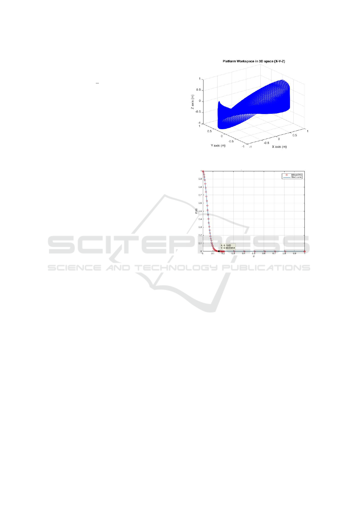
For a person of 1.80m height, using the anthropo-

metric associated data, the deﬁned forward kinematic

model and the range of motion, the workspace is plot-

ted for the three-dimensional space as shown in Fig-

ure 2.

First the penality function P(d) is computed us-

ing equation (26) according to the desired curve data

as explained previously, by using Curve Fitting Pack-

age in Matlab, as depicted in Figure 3. The ob-

tained parameters of the penalty function are given by

: a = 2.5, b = 7.855, p = 100.

Thereby the ﬁnal expression of the penality term

is given by:

P(d) = (sin(2.5d + 7.855))

100

(25)

Figure 2: Workspace for 3D space.

Figure 3: Penality term P(d).

To show the effectiveness of the optimal posture

algorithm, the initial value is ﬁxed in joint space ac-

cording to the feasible biomechanical posture for the

used conﬁguration as q

initguess

= [0, 0,0,0,10,0,0] (in

degree). ˙q

initguess

= [0, 0,0, 0,0, 0,0] and ¨q

initguess

[0,0, 0,0,0,0,0], where the result of the optimization

is usually sensitive to the initial guess.

The remain parameters are given by ε

= ε

= 0.0001, the weight w

for the joints variables of

the lower limb, are deﬁned in (R.T. Marler, 2009).

The optimum kinematic a parapmeters is obtained

using the desired motion in terms of end effector po-

sition, velocity as depicted in Figure 4, which belongs

to the deﬁned workspace, and optimization designed

routine, where the objective function, and constraints

are deﬁned, as described previously.

From the provided checking function, the end-

effector coordinates of desired motion are validated,

and then the optimal position, velocity and accelera-

tion joints are predicted as shown in ﬁgure 5, and 6.

One of the most important factors in the devel-

opment of any optimization problem is the selection

of the suitable ﬁtness function and well deﬁned con-

Optimal 3D Kinematic Analysis for Human Lower Limb Rehabilitation

183

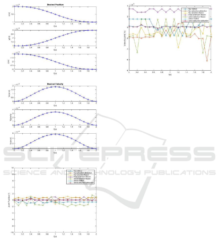
Figure 4: Desired Cartesian-space Trajectory.

Figure 5: Obtained Joint-space Position.

straints according to the problem complexity as de-

scribed in this paper. Using SQP algorithm resolu-

tion for the proposed optimization problem formula-

tion the inverse kinematic model of 3D space human

leg conﬁguration have been predicted, and represent

to our knowledge the ﬁrst study carried out in the all

three plane of human leg conﬁguration.

Figure 6: Obtained Joint-space Velocity.

6 CONCLUSION

A new general optimization-based formulation for op-

timal kinematic analysis for the human lower limb has

been develope, in this study. The proposed method

is developed specialy in three dimensional space, in

terms of the kinematic parameters, using an objective

function incorporating three factors that contribute

to musculoskeletal discomfort as human performance

measure.

The performance measure is referred to the ten-

dency to move sequentially all segments of the hu-

man leg, the tendency to move leg while joints are

near their ROM, and the discomfort associated with

gravitating around a reasonably comfortable position.

This new form of objective function is developed

principally for rehabilitation use, where physiologi-

cal patient constraints need to be taken into consider-

ation.

In this order, according to the physiological con-

straints and the developed forward kinematic model,

the feasible workspace is presented. To validate the

feasability and the effectiveness of the proposed kine-

matic method to predict the inverse kinematic model

of 3D space human leg conﬁguration, a reference tra-

jectory is generated to be suitable in rehabilitation

case, and thereby, applied in the proposed algorithm

solution.

The simulation results, were present an optimal

joint space parameters deﬁning the inverse kinemat-

ics.

However, this study still valid for the static pur-

pose, and can be improved according to a large deﬁni-

tion of discomfort according to dynamical parameters

in term of muscle, fatigue... which can be developed

in the future research.

ICINCO 2017 - 14th International Conference on Informatics in Control, Automation and Robotics

184

ACKNOWLEDGMENT

This work has been supported by Automatic and In-

dustrial Informatics Laboratory (LAII), Ecole Mo-

hammadia dIngenieurs, Mohammed V University,

Rabat, Morocco; Integration of Systems and Ad-

vanced Technologies Laboratory (LISTA), Sciences

Faculty, Fes, Morocco; The Department of Electrical

Engineering, Ecole de Technologie Superieure, Mon-

treal, Canada.

REFERENCES

A. Ochsner, H. A. (2014). Design and computation of mod-

ern engineering materials. In Andreas chsner Holm

Altenbach, Advanced Structured Materials.

Chen, Y. (20004). Changes in lifting dynamics after local-

ized arm fatigue.

C.S. Hernandez, R. S. and Rodrguez, E. (2011). Design and

dynamic modeling of humanoid biped robot e?robot.

In CERMA, Cuernavaca, Mxico.

D. B. Chafﬁn, D. B. J. Anderson, . (1992). Occupational

biomechanics.

Dombre, E. and Khalil, W. (2007). Modeling, Performance

Analysis and Control of Robot Manipulators. Wiley

ISTE.

H. A. Eschenauer, G. T. (1989). Discretization methods and

structural optimization, procedures and applications.

In -Seminar October 5?7, Siegen, FRG.

H. Faqihi, M. Saad, K. B. M. B. and Kabbaj, M. (2016).

Tracking trajectory of a cable-driven robot for lower

limb rehabilitation”, international journal of electri-

cal. International Journal of Electrical, Computer,

Energetic, Electronic and Communication Engineer-

ing, 6(8):1022–1027.

Hogan, N. (1984). An organizing principle for a class of

voluntary movements.

J. M. Porta, L. Ros, F. (2005). Inverse kinematic solution of

robot manipulators using interval analysis.

J. Yang, R. T. Marler, H. K. J. A. K. A.-M. (2004). Multi-

objective optimization for upper body posture predic-

tion. In Albany, NY.

K. Abdel-Malek, J. Yang, W. Y. J. (2004). Human perfor-

mance measures: mathematics.

P. Gill, W. M. and Saunders, A. (2002). Snopt: An sqp

algorithm for large-scale constrained optimization.

Rastegarpanah, A. and Mozafar, S. (2016). Lower limb re-

habilitation using patient data.

R. T. Marler, J. Yang, S. R. K. A.-M.-C. (2009). Use of

multi- objective optimization for digital human pos-

ture prediction.

S. Glowinski, T. K. (Warsaw 2016). An inverse kinematic

algorithm for human leg.

S. Tejomurtula, S. K. (1999). Inverse kinematics in robotics

using neural networks.

S. Tejomurtula, S. K. (2005). Biomechanics and Motor

Control of Human Movement. Wiley, NewYork.

V. Kumar, S. Sen, S. S. D. and Shome, S. (2015). Track-

ing trajectory of a cable-driven robot for lower limb

rehabilitation”, international journal of electrical. In

Proceedings of the 2015 Conference on Advances In

Robotics, India.

W. M. Spong, S. H. and Vidyasagar, M. (2006). Robot mod-

eling and control. ohn Wiley & Sons.

Xie, S. (2016). Advanced Robotics for Medical Rehabilita-

tion.

Z. Mi, Y. Jingzhou, K. A.-M. (2009). Optimization-based

posture prediction for human upper body.

Optimal 3D Kinematic Analysis for Human Lower Limb Rehabilitation

185