Estimating Uncertainty in Time-difference and Doppler Estimates
Gabrielle Flood, Anders Heyden and Kalle
˚
Astr
¨
om
Centre for Mathematical Sciences, Lund University, Lund, Sweden
Keywords:
Time-difference of Arrival, Sub-sample Methods, Doppler Effect, Uncertainty Measure.
Abstract:
Sound and radio can be used to estimate the distance between a transmitter and a sender by correlating the
emitted and received signal. Alternatively by correlating two received signals it is possible to estimate dis-
tance difference. Such methods can be divided into methods that are robust to noise and reverberation, but
give limited precision and sub-sample refinements that are sensitive to noise, but give higher precision when
initialized close to the real translation. In this paper we develop stochastic models that can explain the limits
in the precision of such sub-sample time-difference estimates. Using such models we provide new methods
for precise estimates of time-differences as well as Doppler effects. The method is verified on both synthetic
and real data.
1 INTRODUCTION
Audio and radio sensors are becoming ubiquitous
among our everyday tools, e.g. smartphones, laptops,
and tablet pc’s. They also form the backbone of
internet-of-things, e.g. small low-power units that can
run for years on batteries or use energy harvesting to
run for extended periods. Given the location of each
one of these units, it is possible to use them as an ad-
hoc acoustic sensor network. Such sensor networks
can be used for many interesting applications. One
use-case is localization, cf. (Brandstein et al., 1997;
Cirillo et al., 2008; Cobos et al., 2011; Do et al.,
2007). Another application is to improve the sound
quality using so called beam-forming, (Anguera et al.,
2007). A third application is so called speaker di-
arization, i.e. to determine who spoke when, (Anguera
et al., 2012). If the sensor positions are unknown or
only known to a certain accuracy, the results of such
applications are inferior as is shown in (Plinge et al.,
2016). However, even without any prior information
it is possible to estimate both sender and receiver po-
sitions up to a choice of coordinate system, (Polle-
feys and Nister, 2008; Crocco et al., 2012; Kuang
et al., 2013; Kuang and
˚
Astr
¨
om, 2013a; Zhayida et al.,
2014), thus providing accurate sensor positions. A
key component for all of these methods is the pro-
cess of obtaining features such as time-difference es-
timates from pairwise channels. In this paper we will
primarily focus on sound. However the same princi-
ples are applicable for radio (Batstone et al., 2016).
1
2
3
4
5
6
7
8
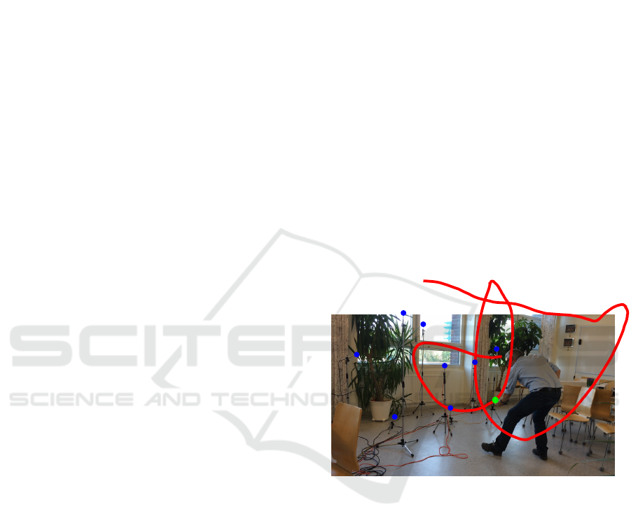
Sound source
Microphones
P
r
o
j
e
c
t
e
d
3
D
p
a
t
h
Figure 1: Precise time-difference of arrival estimation can
be used for many purposes, e.g. beam-forming, diarization,
anchor free node calibration and positioning. The figure
illustrates its use for anchor free node calibration, sound
source movement and room reconstruction.
All of these applications depend on accurate ways
of comparing the sound (or radio) signals so as to
extract information. The most common approach is
to estimate time-differences, which are then used for
subsequent processing. For the applications it is of
interest to obtain the most precise estimate possible.
In (Zhayida and
˚
Astr
¨
om, 2016) sub-sample methods
were used to improve on the time-difference estimates
and it is empirically shown to give better estimates of
the receiver-sender configurations. However, no anal-
ysis of the sub-sample time-difference uncertainties
was provided.
Flood, G., Heyden, A. and Åström, K.
Estimating Uncertainty in Time-difference and Doppler Estimates.
DOI: 10.5220/0006722002450253
In Proceedings of the 7th International Conference on Pattern Recognition Applications and Methods (ICPRAM 2018), pages 245-253
ISBN: 978-989-758-276-9
Copyright © 2018 by SCITEPRESS – Science and Technology Publications, Lda. All rights reserved
245

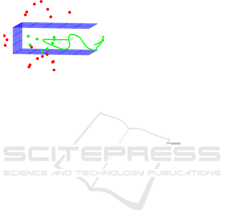
Mirrored microphones
Figure 2: The figure examplifies one usage of precise time-
difference of arrival estimation. The image illustrates the
estimated microphone positions (green dots), estimated mir-
rored microphone positions (red dots) and sound source
motion (green curve) from Fig 1. The estimated reflective
planes are also shown in the figure. These three planes cor-
respond to the floor, the ceiling and the wall.
The main contributions of this paper are:
• A framework for estimating time-difference es-
timates and for estimating the precision of such
time-difference estimates.
• An extension of the method to also estimate
minute Doppler effects.
• In practice there is also significant difference in
amplitude of the signals. Accurate results require
that also these amplitude changes are estimated
and accounted for.
• A synthetic evaluation that demonstrates both the
validity of the models, but also provides knowl-
edge on the failure modes of the method.
• Evaluation on real data that demonstrate that
there is useful information not only in the time-
difference estimates but also in the amplitude
changes and in the minute Doppler effects, even
for speeds as small as 0.1 m/s.
2 MODELING PARADIGM
2.1 Measurement and Error Model
In this paper, we study discretely sampled signals,
such as audio signals. We assume that signals have
been sampled at a fixed and known sampling rate. A
reasonable measurement model is that the measured
signal y is the result of ideal sampling and added
noise, i.e.
y(k) = Y (k) +e(k) . (1)
Here Y : R 7→ R is the original, continuous signal and
e is a discrete stationary stochastic process.
Let B denote the set of continuous functions
Y : R → R that are also square integrable and such
that the Fourier transform is zero outside the inter-
val [−π,π]. Let ` denote the set of discrete func-
tions y : Z → R that are also square integrable. For
such functions we introduce the discretization opera-
tor D : B → `, such that
y(i) = D(Y )(i) = Y (i).
We also introduce the interpolation operator I
g
:
` → B, such that
Y (x) = I
g
(y)(x) =
∞
∑
i=−∞
g(x −i)y(i).
The ideal interpolation operator I : ` → B is in-
terpolation using the normalized sinc function, with
g(x) = sinc(x). We have that ideal interpolation re-
stores the sampled function, (Shannon, 1949), i.e.
I(D(Y )) = Y .
Other interpolation methods can often be written
in a similar way. E.g. by substituting sinc by
G
a
(x) =
1
√
2πa
2
e
x
2
/2a
2
we get Gaussian interpolation.
2.2 Scale-space Smoothing and Ideal
Interpolation
The measured and interpolated signal can be
smoothed to decrease the impact of measurement
noise. This also makes it easier to capture patterns
on a coarser scale, (Lindeberg, 1994). We have used
a Gaussian kernel G
a
2
, with standard deviation a
2
, for
the smoothing. Later, a
2
will also be referred to as the
smoothing parameter.
Given a sampled signal y, the ideally interpolated
and smoothed signal can be expressed
Y (x) = (G
a
2
∗I
sinc
(y))(x) = I
G
a
2
∗sinc
(y)(x).
For a sufficiently large a
2
we have G
a
2
∗sinc ≈
G
a
2
. Thus ideal interplation followed by Gaussian
smoothing can be approximated to interpolation us-
ing the Gaussian (
˚
Astr
¨
om and Heyden, 1999), s.t.
Y (x) = I
G
a
2
∗sinc
(y)(x) ≈ (I
G
a
2
(y))(x). (2)
What sufficiently large means will be discussed later,
in Section 4.1.
Furthermore we will use that discrete w.s.s. Gaus-
sian noise interpolates to continuous w.s.s. Gaussian
noise and vice versa, as is shown in (
˚
Astr
¨
om and Hey-
den, 1999).
ICPRAM 2018 - 7th International Conference on Pattern Recognition Applications and Methods
246

3 TIME-DIFFERENCE AND
DOPPLER ESTIMATION
Assume that we have two signals, W (t) and
¯
W (t). The
signals are measured and interpolated as described in
the previous section. Also assume that the two signals
are similar, but not identical. This can e.g. arise when
a single audio signal is picked up by two different re-
ceivers. Then, one of the signals can be described by
the other and a few parameters. We describe the rela-
tion as follows
W (t) =
¯
W (αt + h). (3)
Here, h is a translation or the time-difference of ar-
rival. If the distances from the sound source to the
two microphones are the same, h = 0. The second pa-
rameter, α, is a Doppler factor. This is interesting if
either the sound source or the microphones are mov-
ing. For a stationary setup α = 1.
When the two signals are picked up by the micro-
phones they are disturbed by Gaussian w.s.s. noise.
Thus, the received signals are better described by
V (t) = W (t) + E(t),
¯
V (t) =
¯
W (t) +
¯
E(t) , (4)
where E(t) and
¯
E(t) denotes the two independent
noise signals after interpolation.
Now, assume that the signals V and
¯
V are given.
Also, denote z
z
z =

z
1
z
2

T
=

h α

T
. Then, the
parameters for which (3) is true can be estimated by
the z
z
z that minimizes the integral
F(z
z
z) =
Z
t
(V (t) −
¯
V (z
2
t + z
1
))
2
dt . (5)
3.1 Estimating Standard Deviation of
the Parameters
If z
z
z
T
=

h
T
α
T

T
is the true parameter and
ˆ
z
z
z is the
parameter that has been estimated by (5), the estima-
tion error can be expressed as
X =
ˆ
z
z
z −z
z
z
T
.
Assume, without loss of generality, that z
z
z
T
=

0 1

T
. The standard deviation of
ˆ
z
z
z will be the same
as the standard deviation of X and the mean of those
two will only differ by z
z
z
T
. Thus, we can study X to
get statistical information about
ˆ
z
z
z.
Linearizing F(z
z
z) around the true displacement
z
z
z
T
=

0 1

T
we get
F(X) =
1
2
X
T
aX +bX + f ,
with
a = ∇
2
F(z
z
z
T
), b = ∇F(z
z
z
T
), f = F(z
z
z
T
).
Using (4) and (3), this gives
f =F(

0 1

T
) =
Z
t
(V (t) −
¯
V (1 ·t −0))
2
dt
=
Z
t
(W (t) + E(t) −(
¯
W (t) +
¯
E(t)))
2
dt
=
Z
t
(E −
¯
E)
2
dt =
Z
t
E
2
+ 2E
¯
E +
¯
E
2
dt.
Straightforward calculations give
b = −2

R
t
ˆ
ϕdt
R
t
t
ˆ
ϕdt

,
with
ˆ
ϕ = E
¯
W
0
+ E
¯
E
0
−
¯
E
¯
W
0
−
¯
E
¯
E
0
.
Furthermore,
∇
2
F =

R
t
φdt
R
t
tφdt
R
t
tφdt
R
t
t
2
φdt

,
using
φ(z
z
z) = (
¯
V
0
(αt + h))
2
−
V (t)
¯
V
00
(αt + h) +
¯
V (αt + h)
¯
V
00
(αt + h).
If we let
ˆ
φ =φ(z
z
z
T
) = (
¯
W
0
(t) +
¯
E
0
(t))
2
−(W(t) + E(t))(
¯
W
00
(t) +
¯
E
00
(t))
+ (
¯
W (t) +
¯
E(t))(
¯
W
00
(t) +
¯
E
00
(t))
=(
¯
W
0
)
2
+ 2
¯
W
0
¯
E
0
+ (
¯
E
0
)
2
−E
¯
W
00
−E
¯
E
00
+
¯
E
¯
W
00
+
¯
E
¯
E
00
we get
a = ∇
2
F(z
z
z
T
) =

R
t
ˆ
φdt
R
t
t
ˆ
φdt
R
t
t
ˆ
φdt
R
t
t
2
ˆ
φdt

.
We have that F(X ) = 1/2 ·X
T
aX + bX + f . To
minimize this function, one should find the X for
which the derivative of F(X) is zero.
∇F(X) = aX + b = 0 ⇔ X = g(a, b) = −a
−1
b.
In the calculations we will assume that a is invertible.
Now we want to find the mean and covariance of
X. For this, Gauss’ approximation formula is used.
If we denote the expected value of a and b with µ
a
=
E[A] and µ
b
= E[b] respectively the expected value of
X can be approximated to
E[X] =E[g(a,b)] ≈ E[g(µ
a
,µ
b
) + (a −µ
a
)g
0
a
(µ
a
,µ
b
)
+ (b −µ
b
)g
0
b
(µ
a
,µ
b
)]
=g(µ
a
,µ
b
) + (E[a] −µ
a
)g
0
a
(µ
a
,µ
b
)
+ (E[b] −µ
b
)g
0
b
(µ
a
,µ
b
)
=g(µ
a
,µ
b
) = −µ
−1
a
µ
b
= −E[a]
−1
E[b].
(6)
Estimating Uncertainty in Time-difference and Doppler Estimates
247

In the same manner the covariance of X is
C[X] =C[g(a,b)] ≈g
0
a
(µ
a
,µ
b
)
T
C[a]g
0
a
(µ
a
,µ
b
)
+ g
0
b
(µ
a
,µ
b
)
T
C[b]g
0
b
(µ
a
,µ
b
)
+ 2g
0
a
(µ
a
,µ
b
)
T
C[a,b]g
0
b
(µ
a
,µ
b
),
(7)
where C[a,b] denotes the cross-covariance between a
and b. For further computations g
0
a
(a,b) = −(a
−1
)
2
b,
g
0
b
(a,b) = −a
−1
, E[a], E[b], C[b] and C[a,b] are
needed.
By computing the expected value of
ˆ
ϕ
E[
ˆ
ϕ] =E[E
¯
W
0
+ E
¯
E
0
−
¯
E
¯
W
0
−
¯
E
¯
E
0
]
=E[E]
¯
W
0
+ E[E]E[
¯
E
0
] −E[
¯
E]
¯
W
0
−E[
¯
E]E[
¯
E
0
]
=0
we get
E[b] =E

−2

R
t
ˆ
ϕ dt
R
t
t
ˆ
ϕdt

= −2

R
t
E[
ˆ
ϕ]dt
R
t
tE[
ˆ
ϕ]dt

= −2

R
t
0dt
R
t
t ·0 dt

=

0
0

.
In the second step of the computation of E[
ˆ
ϕ] we have
used that for a weakly stationary process the process
and its derivative at a certain time are uncorrelated,
and thus E[
¯
E
¯
E
0
] = E[
¯
E]E[
¯
E
0
], (Lindgren et al., 2013).
Hence,
E[X] = −E[a]
−1
E[b] = −E[a]
−1

0
0

=

0
0

.
Since E[b] = 0
0
0, we get that g
0
a
(µ
a
,µ
b
) = 0
0
0. Thus
the first and the last term in (7) cancel, leaving
C[X] =g
0
b
(µ
a
,µ
b
)
T
C[b]g
0
b
(µ
a
,µ
b
)
=(−E[a]
−1
)
T
C[b](−E[a]
−1
)
=(E[a]
−1
)
T
C[b]E[a]
−1
.
(8)
To find the expected value of a we need the ex-
pected value of
ˆ
φ. This is
E[
ˆ
φ] =(
¯
W
0
)
2
+ 2
¯
W
0
E[
¯
E
0
] + E[(
¯
E
0
)
2
] −
¯
W
00
E[E]
−E[E]E[
¯
E
00
] +
¯
W
00
E[
¯
E] + E[
¯
E
¯
E
00
]
=(
¯
W
0
)
2
+ E[(
¯
E
0
)
2
] + E[
¯
E
¯
E
00
] = (
¯
W
0
)
2
.
In the last equality we have used that E[
¯
E
¯
E
00
] =
−E[(
¯
E
0
)
2
], (Lindgren et al., 2013). Thus, the two last
terms cancel. The expected value of a is therefore
E[a] =2

R
t
E[
ˆ
φ]dt
R
t
E[t
ˆ
φ]dt
R
t
E[t
ˆ
φ]dt
R
t
E[t
2
ˆ
φ]dt

=2

R
t
(
¯
W
0
)
2
dt
R
t
t(
¯
W
0
)
2
dt
R
t
t(
¯
W
0
)
2
dt
R
t
t
2
(
¯
W
0
)
2
dt

.
Now, since the expected value of b is zero, the
covariance of b is
C[b] = (−2)
2

C
11
C
12
C
21
C
22

,
with
C
11
= E

Z
t
1
ˆ
ϕ(t
1
)dt
1
·
Z
t
2
ˆ
ϕ(t
2
)dt
2

C
12
= E

Z
t
1
t
1
ˆ
ϕ(t
1
)dt
1
·
Z
t
2
ˆ
ϕ(t
2
)dt
2

C
21
= E

Z
t
1
ˆ
ϕ(t
1
)dt
1
·
Z
t
2
t
2
ˆ
ϕ(t
2
)dt
2

C
22
= E

Z
t
1
t
1
ˆ
ϕ(t
1
)dt
1
·
Z
t
2
t
2
ˆ
ϕ(t
2
)dt
2

.
Note that by changing the order of the terms in C
21
it
is clear that C
21
= C
12
. Furthermore we get
C
11
=E

Z
t
1
ˆ
ϕ(t
1
)dt
1
·
Z
t
2
ˆ
ϕ(t
2
)dt
2

=E
h
Z
t
1
(E −
¯
E)(
¯
W
0
+
¯
E
0
)dt
1

·

Z
t
2
(E −
¯
E)(
¯
W
0
+
¯
E
0
)dt
2
i
=E
h
Z
t
1
Z
t
2
(E(t
1
) −
¯
E(t
1
))(
¯
W
0
(t
1
) +
¯
E
0
(t
1
))
·(E(t
2
) −
¯
E(t
2
))(
¯
W
0
(t
2
) +
¯
E
0
(t
2
))dt
1
dt
2
i
.
Denoting E[(E(t
1
) −
¯
E(t
1
))(E(t
2
) −
¯
E(t
2
))] =
r
E−
¯
E
(t
1
−t
2
) and assuming that E[
¯
E
0
(t
1
)
¯
E
0
(t
2
)] is
small yields
C
11
=E

Z
t
1
ˆ
ϕ(t
1
)dt
1
·
Z
t
2
ˆ
ϕ(t
2
)dt
2

=
Z
t
1
Z
t
2
E[(E(t
1
) −
¯
E(t
1
))(E(t
2
) −
¯
E(t
2
))]
·(
¯
W
0
(t
1
)
¯
W
0
(t
2
)
+
¯
W
0
(t
1
)E[
¯
E
0
(t
2
)] + E[
¯
E
0
(t
1
)]
¯
W
0
(t
2
)
+ E[
¯
E
0
(t
1
)
¯
E
0
(t
2
)])dt
2
dt
1
≈
Z
t
1
Z
t
2
r
E−
¯
E
(t
1
−t
2
)
¯
W
0
(t
1
)
¯
W
0
(t
2
)dt
2
dt
1
=
Z
t
1
¯
W
0
(t
1
)(
¯
W
0
∗r
E−
¯
E
)(t
1
)dt
1
.
The time t is not stochastic and the other elements in
C[b] can be computed similarly. Finally
C
11
=
Z
t
¯
W
0
(t)(
¯
W
0
∗r
E−
¯
E
)(t)dt
C
12
= C
21
=
Z
t
t
¯
W
0
(t)(
¯
W
0
∗r
E−
¯
E
)(t)dt
C
22
=
Z
t
t
¯
W
0
(t)((t
¯
W
0
) ∗r
E−
¯
E
)(t)dt
and through (8) an expression for the variance and
thus also the standard deviation of X is found.
ICPRAM 2018 - 7th International Conference on Pattern Recognition Applications and Methods
248

-5
-4
-3
-2
-1
0
1
2
3
4
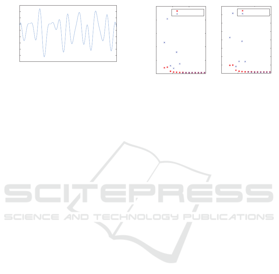
Figure 3: The simulated signal that was used for the experi-
mental validation. Later, noise of different levels was added
to achieve a more realistic signal.
3.2 Expanding the Model
The model (3) can easily be changed or expanded to
contain more (or fewer) parameters. One example is
the addition of an amplitude parameter γ, such that
W (t) = γ
¯
W (αt + h). (9)
The integral (5) would then be changed accord-
ingly and one would instead optimize over z
z
z =

z
1
z
2
z
3

=

h α γ

.
In practice, the parameter computations will not
be harder for more parameters. However the analy-
sis carried out in the previous section does get more
complex.
4 EXPERIMENTAL VALIDATION
For validation we use both synthetic data and real
data. When we use synthetic data, the purpose is both
to demonstrate the validity of the model and the ap-
proximations, but also to explore at what signal-to-
noise ratio the approximations no longer hold. For
the real data experiments, the purpose is to show that
there is useful information in the estimated parame-
ters. For time-difference this is well-known, but for
the Doppler effects it is less known.
4.1 Synthetic Data - Validation of
Method
Initially we tested the model on simulated data. This
was done to investigate when the approximations in
the model are valid. Examples of such are the lin-
earization from Gauss’ approximation formula, e.g.
(3.1) and (7), and that ideal interpolation followed by
convolution with a Gaussian can be approximated to
Gaussian interpolation (2).
To do this we compared the theoretical standard
deviations of the parameters calculated according to
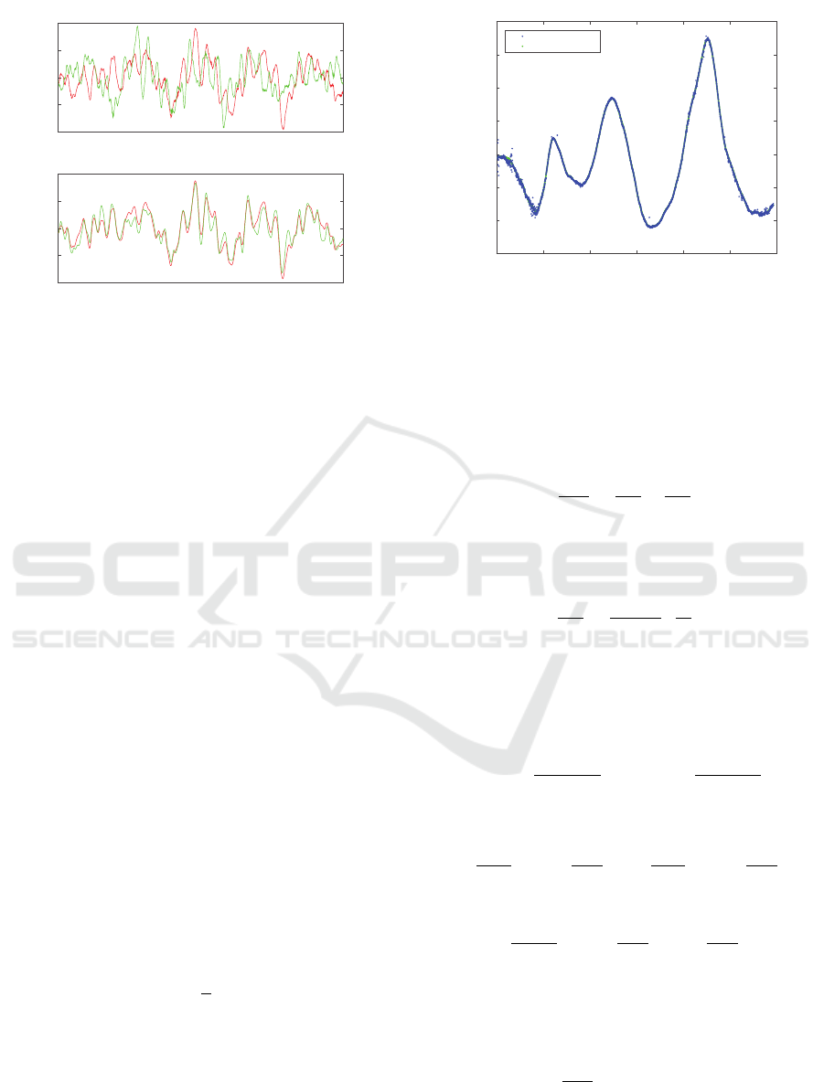
0.2 0.4 0.6 0.8
a
2
0
0.5
1
1.5
2
2.5
σ
Theoretical std
Empirical std
h
0.2 0.4 0.6 0.8
a
2
0
0.5
1
1.5
2
2.5
3
3.5
4
σ
α
×10
-3
Theoretical std
Empirical std
Figure 4: The plots show the standard deviation of the pa-
rameters in z
z
z for different values of the smoothing param-
eter a
2
. The red stars (∗) represent the theoretical values
σ
z
z
z
and the blue crosses (x) the empirical values
ˆ
σ
z
z
z
. The
left plot shows the results for the translation z
1
= h and the
right plot for the Doppler factor z
2
= α. It is clear that the
approximation is valid approximately when a
2
> 0.55.
Section 3.1 with empirically computed standard de-
viations. While these agree our approximations are
assumed to be valid.
An original continuous signal W(x) was simu-
lated, see Fig 3. The second signal was created ac-
cording to (3) s.t.
¯
W = W(1/α ·(x −h)). Thereafter
both signals were ideally sampled and then Gaussian
white discrete noise with standard deviation σ
n
was
added to the discrete signals. During the analysis
both signals were interpolated using a Gaussian ker-
nel with standard deviation a
2
, according to Section
2.2. At this point the signals could be described by
V (t) and
¯
V (t) as before.
To study the effect of a
2
and σ
n
the signals V and
¯
V were re-simulated 1000 times using the same orig-
inal signals W and
¯
W , but different noise. The the-
oretical standard deviation of the parameter vector z
z
z,
σ
z
z
z
=

σ
h
σ
α

, was then computed according to the
presented theory, while the empirical standard devi-
ation,
ˆ
σ
z
z
z
=

ˆ
σ
h
ˆ
σ
α

, was computed from the 1000
achieved parameter estimations.
First the effect of changing a
2
was studied. The
noise level was set to σ
n
= 0.03, the translation was
h = 3.63 and the Doppler factor was set to α = 1.02 –
though the actual numbers are not of importance. The
standard deviation of z
z
z was then computed according
to above. This was done for several different a
2
∈
[0.3,0.8].
The results are shown in Fig 4. It can be seen
that the theoretical and empirical values σ
z
z
z
and
ˆ
σ
z
z
z
disagree for both parameters when a
2
is lower than
a
2
≈ 0.55. Thus the approximation (2) of ideal inter-
polation should only be used for a smoothing param-
eter a
2
> 0.55.
Secondly we investigated the impact of the noise.
Estimating Uncertainty in Time-difference and Doppler Estimates
249

0 0.2 0.4 0.6 0.8 1 1.2 1.4 1.6
σ
0
0.5
1
1.5
2
2.5
σ
Theoretical std
Empirical std
n
h
0 0.2 0.4 0.6 0.8 1 1.2 1.4 1.6
σ
0
1
2
3
4
5
6
σ
α
×10
-3
Theoretical std
Empirical std
n
Figure 5: The standard deviation of the translation (on top)
and Doppler factor (bottom) for different levels of noise in
the signal. The red stars (∗) mark the theoretical values σ
z
z
z
and the blue crosses (x) the empirical
ˆ
σ
z
z
z
. For the translation
the values agree for signals with a noise level up to σ
n
≈
0.8. For the Doppler factor the theoretical values follow the
empirical values for σ
n
< 1.1.
The smoothing parameter was now fixed at a
2
= 2 and
the translation and the Doppler factor were again set
to h = 3.63 and α = 1.02. Then σ
z
z
z
and
ˆ
σ
z
z
z
were com-
puted as before. This time it was done for several
different σ
n
∈ [0,1.6].
The results are shown in Fig 5. The uppermost
plot contains the results for the translation parame-
ter h and the plot below the corresponding results for
the Doppler parameter α. Each plot shows the stan-
dard deviation of the parameter for different levels of
noise. The theoretical and empirical standard devi-
ation of the translation agree for values lower than
σ
n
≈ 0.8, after which they start to differ. Concern-
ing the Doppler factor the theoretical and empirical
values agree well until σ
n
≈ 1.1, after which the esti-
mation is poor.
Thus, by studying the plots we can conclude that
the system can handle noise with a standard deviation
up to σ
n
≈ 0.8. The amplitude for the original signal
varies between 1 and 3.5. Using the standard devi-
ation of the original signal, σ
W
, the signal-to-noise
ratio is
SNR =
σ
2
n
σ
2
W
≈ 0.21.
4.2 Real Data - Validation of Method
For the real data experiments we used 8 T-Bone MM-
1 microphones, connected to an audio interface (M-
Audio Fast Track Ultra 8R), which was connected
to a computer. The sound was recorded at f = 96
kHz and we made the experiments in an anaechoic
chamber. The eight microphones were placed approx-
imately 0.3-1.5 meters away from each other and so
that they spanned 3D. We generated sounds by play-
ing a song on a mobile phone connected to a simple
loudspeaker, while moving around in the room.
Using the sound generated from all eight micro-
phones we estimated the sound source path, i.e. a 3D
trajectory s(t) and the eight 3D positions of the mi-
crophones r
1
,...,r
8
. This was done using the tech-
nique described in (Zhayida et al., 2014) and re-
fined in (Zhayida et al., 2016). The method builds
on RANSAC algorithms based on minimal solvers
(Kuang and
˚
Astr
¨
om, 2013b) to find initial estimates
of the sound trajectory s(t) and microphone positions
r
1
,...,r
8
. These estimates are then refined using non-
linear optimization of a robust error norm, but also
including a smooth motion prior.
For the validation of the method presented in this
article we used data from two of the microphones.
The played song lasted for approximately 29 s and the
loudspeaker moved during the whole time. Further-
more, the motion was not constant – both the speed
and direction were changed.
Since our method assume a constant parameter z
in a window the recording was divided into patches
for which the parameters were approximately con-
stant. We divided the signal into 2834 patches of 1000
samples (i.e. approximately 0.01 s) each. Each of
these patches was then investigated separately. For
each patch i a constant loudspeaker position was
given from ground truth. Thus, we had one sender
position s
(i)
, its derivative
∂s
(i)
∂t
(i) and two receiver po-
sitions r
1
and r
2
to compare our results with.
4.2.1 Estimating the Parameters
As mentioned in Section 3.2 it is in practice not harder
to estimate three model parameters. Therefore, to get
a more precise solution, we have used (9) as model for
the received signals. In this case V
(i)
(t) will be signal
patch i from the first microphone and
¯
V
(i)
(t) the cor-
responding signal patch from the second microphone.
Our method is developed to estimate small trans-
lations, s.t. h ∈ [−10,10] samples and the delays in
the experiments were larger than that. Therefore we
pre-estimated the translation using GCC-PHAT. For
a description of the method, see (Knapp and Carter,
1976). The pre-estimation gave an integer delay
˜
h
(i)
,
whereas our method did a subsample refinement, es-
timated the Doppler parameter and the amplitude fac-
ICPRAM 2018 - 7th International Conference on Pattern Recognition Applications and Methods
250

-4
-2
0
2
4
×10
-3
-4
-2
0
2
4
×10
-3
Figure 6: One example of the received signal patches at a
certain time – the first signal in red and the second in green.
The top image shows the signals before any modification.
The bottom image shows the same patches after modifica-
tions using the optimal parameters.
tor. This was done by minimizing the intergral
Z
t
(V
(i)
(t) −γ
(i)
¯
V
(i)
(α
(i)
t +
˜
h
(i)
+ h
(i)
))
2
dt.
Note that
˜
h
(i)
should be viewed as a constant in the
equation above, while we were optimizing over h
(i)
,
α
(i)
and γ
(i)
.
This optimization was performed for all different
patches. The result from one of these can be seen in
Fig 6.
4.2.2 Comparing to Ground Truth
Using r
1
, r
2
and s
(i)
we calculated the distances d
(i)
1
and d
(i)
2
from the loudspeaker to the microphones,
d
(i)
1
= |r
1
−s
(i)
|, d
(i)
2
= |r
2
−s
(i)
|.
The difference between these two distances, ∆d
(i)
=
d
(i)
2
−d
(i)
1
, is connected to the time difference of ar-
rival, and thus our computed translation h
(i)
. While
h
(i)
in measured in samples, ∆d
(i)
is a measure in me-
ters. Thus, we multiplied h
(i)
with a scaling factor
c/ f , where c = 340 m/s is the speed of sound and
f = 96 kHz is the recording frequency. By that we
had an estimation of ∆d
(i)
,
∆d
(i)
=
c
f
·h
(i)
.
In a similar manner the time in samples can be ex-
pressed in seconds using f . Thereafter we could com-
pare our estimation to ground truth. In Fig 7 ground
truth ∆d
(i)
is plotted together with our estimations for
all patches, i.e. over time. It is clear that these agree
well.
0 5 10 15 20 25 30
time [s]
-0.8
-0.6
-0.4
-0.2
0
0.2
0.4
0.6
d
2
-d
1
[m]
Our results
Ground truth
Figure 7: The figure shows the difference between the dis-
tances from receiver 1 to the sender (d
1
) and receiver 2 to
the sender (d
2
) over time. Each dot represents the value for
one signal patch. The ground truth is plotted in green and
our estimations in blue. It is hard to distinguish any green
dots since the estimations agree well with ground truth.
Concerning the Doppler parameter this is a mea-
sure of the change of distance differences, i.e.
∂∆d
∂t
=
∂d
2
∂t
−
∂d
1
∂t
.
Here d
1
and d
2
denotes the distances over time, i.e.
for all patches. If we look at one of the derivatives we
have that d
1
(t) = |r
1
−s(t)| and
∂d
1
∂t
=
r
1
−s
|r
1
−s|
·
∂s
∂t
,
where · denotes the scalar product between the two
time dependent vectors. The derivative of d
2
is found
similarly. Let n
(i)
1
and n
(i)
2
be unit vectors in the direc-
tion from s
(i)
to r
1
and r
2
respectively, i.e.
n
(i)
1
=
r
1
−s
(i)
|r
1
−s
(i)
|
, n
(i)
2
=
r
2
−s
(i)
|r
2
−s
(i)
|
.
Then, for a certain time step, the derivatives will be
∂d
(i)
1
∂t
= n
(i)
1
·
∂s
(i)
∂t
,
∂d
(i)
2
∂t
= n
(i)
2
·
∂s
(i)
∂t
and thus
∂∆d
(i)
∂t
= n
(i)
2
·
∂s
(i)
∂t
−n
(i)
1
·
∂s
(i)
∂t
.
These ground truth Doppler values show how
much ∆d changes each second. However, our esti-
mated Doppler factor α is a unitless constant. The
relation between the two values is
∂∆d
∂t
= (α −1) ·c,
with c still denoting the speed of sound. In Fig 8 we
have plotted the ground truth value in green together
Estimating Uncertainty in Time-difference and Doppler Estimates
251

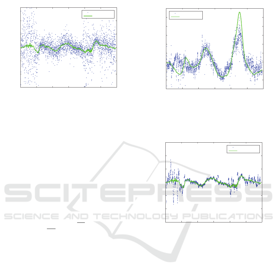
0 5 10 15 20 25 30
time [s]
-3
-2
-1
0
1
2
3
∂ ∆d/
∂ t [m/s]
Our results
Ground truth
Figure 8: The derivative of the distance differences ∆d plot-
ted over time. The blue dots are our estimations and the
solid green line is computed from ground truth. We see
that even though the estimations are noisy they agree with
ground truth.
with our estimations in blue. Even though the estima-
tions are noisy the pattern and the similarities are well
distinguishable.
There is also a relation between the amplitude fac-
tor for the two received signals and the distances d
(i)
1
and d
(i)
2
. Our estimated amplitude γ
(i)
should be re-
lated to the distance quotient d
(i)
2
/d
(i)
1
. Furthermore,
the sound from the loudspeaker spreads as on the sur-
face of a sphere. Thus, the distance quotient is pro-
portional to the square root of the amplitude γ
(i)
,
d
(i)
2
d
(i)
1
= C ·
q
γ
(i)
.
We estimated the proportionality constant using data
and got C = 1.3.
The distance quotient is plotted over time in Fig 9
– our estimations as blue dots and ground truth as a
green line. Again we see that they clearly follow the
same pattern.
The results from above show that our estimated
parameters do contain relevant information. Though,
the estimations in Fig 7, 8 and 9 are all quite noisy.
This can be reduced by computing a moving aver-
age of the estimations. Fig 10 is similar to Fig 8 but
instead of plotting the estimated derivative for each
patch we have plotted the 20-patch moving average
of the distance difference derivative. This means we
have averaged over approximately 0.2 s. A compar-
ison between the two figures shows that the moving
average substantially reduces the noise in the esti-
mates. The same method can be applied to the es-
timations of the translation h and the amplitude γ to
reduce noise.
0 5 10 15 20 25 30
time [s]
0.6
0.7
0.8
0.9
1
1.1
1.2
1.3
1.4
1.5
d
2
/d
1
Our results
Ground truth
Figure 9: The distance quotient d
2
/d
1
plotted over time.
The green solid line represents the ground truth and each
blue dot is the estimation for a certain patch. While the
estimations are somewhat noisy there is no doubt that the
pattern is the same.
0 5 10 15 20 25 30
time [s]
-3
-2
-1
0
1
2
3
∂ ∆d/∂ t [m/s]
Our results
Ground truth
Figure 10: This plot shows essentially the same thing as
Fig 8, i.e. ∂∆d/∂t, but with a 20-patches moving average
over the estimations. The averaging substantially reduces
the noise.
Still after averaging, the estimations are noisy and
poor in the beginning of the signal. This can be ex-
plained by the song that was played. The song starts
with occasional drum beats with silence in between.
Since the sound is not persistent the information is not
sufficient to make good estimates. When the song is
more continuous, after 5-6 s, this shows as the esti-
mates get better.
5 CONCLUSIONS
In this paper we study the estimation of time-
differences, amplitude changes and minute Doppler
effects from two signals. We also study how to esti-
mate the uncertainty in these estimated parameters.
ICPRAM 2018 - 7th International Conference on Pattern Recognition Applications and Methods
252

The results are useful both for simultaneous determi-
nation of sender and receiver positions, but also for
localization, beam-forming and diarization. In the pa-
per we use previous results on stochastic analysis of
interpolation and smoothing in order to give explicit
formulas for the covariance matrix of the estimated
parameters. We show that the approximations used
are valid as long as the smoothing is at least 0.55 sam-
ple points and as long as the signal-to-noise ratio is
smaller than 0.21. Furthermore we show in experi-
mental studies on real data that these estimates pro-
vide useful information for subsequent analysis.
ACKNOWLEDGEMENTS
This work is supported by the strategic research
projects ELLIIT and eSSENCE, Swedish Foundation
for Strategic Research project ”Semantic Mapping
and Visual Navigation for Smart Robots” (grant no.
RIT15-0038) and Wallenberg Autonomous Systems
and Software Program (WASP).
REFERENCES
Anguera, X., Bozonnet, S., Evans, N., Fredouille, C., Fried-
land, G., and Vinyals, O. (2012). Speaker diarization:
A review of recent research. IEEE Transactions on
Audio, Speech, and Language Processing, 20(2):356–
370.
Anguera, X., Wooters, C., and Hernando, J. (2007). Acous-
tic beamforming for speaker diarization of meetings.
IEEE Transactions on Audio, Speech, and Language
Processing, 15(7):2011–2022.
˚
Astr
¨
om, K. and Heyden, A. (1999). Stochastic analysis of
scale-space smoothing. Advances in Applied Proba-
bility, 30(1).
Batstone, K., Oskarsson, M., and
˚
Astr
¨
om, K. (2016). Ro-
bust time-of-arrival self calibration and indoor local-
ization using wi-fi round-trip time measurements. In
proc. of International Conference on Communication.
Brandstein, M., Adcock, J., and Silverman, H. (1997). A
closed-form location estimator for use with room en-
vironment microphone arrays. Speech and Audio Pro-
cessing, IEEE Transactions on, 5(1):45 –50.
Cirillo, A., Parisi, R., and Uncini, A. (2008). Sound map-
ping in reverberant rooms by a robust direct method.
In Acoustics, Speech and Signal Processing, IEEE In-
ternational Conference on, pages 285 –288.
Cobos, M., Marti, A., and Lopez, J. (2011). A modi-
fied SRP-PHAT functional for robust real-time sound
source localization with scalable spatial sampling.
Signal Processing Letters, IEEE, 18(1):71 –74.
Crocco, M., Del Bue, A., Bustreo, M., and Murino, V.
(2012). A closed form solution to the microphone po-
sition self-calibration problem. In ICASSP.
Do, H., Silverman, H., and Yu, Y. (2007). A real-time SRP-
PHAT source location implementation using stochas-
tic region contraction(SRC) on a large-aperture micro-
phone array. In ICASSP 2007, volume 1, pages 121–
124.
Knapp, C. and Carter, G. (1976). The generalized correla-
tion method for estimation of time delay. IEEE Trans-
actions on Acoustics, Speech and Signal Processing,
24(4):320–327.
Kuang, Y. and
˚
Astr
¨
om, K. (2013a). Stratified sensor net-
work self-calibration from tdoa measurements. In EU-
SIPCO.
Kuang, Y. and
˚
Astr
¨
om, K. (2013b). Stratified sensor net-
work self-calibration from tdoa measurements. In 21st
European Signal Processing Conference 2013.
Kuang, Y., Burgess, S., Torstensson, A., and
˚
Astr
¨
om, K.
(2013). A complete characterization and solution to
the microphone position self-calibration problem. In
ICASSP.
Lindeberg, T. (1994). Scale-space theory: A basic tool for
analyzing structures at different scales. Journal of ap-
plied statistics, 21(1-2):225–270.
Lindgren, G., Rootz
´
en, H., and Sandsten, M. (2013). Sta-
tionary Stochastic Processes for Scientists and Engi-
neers. CRC Press.
Plinge, A., Jacob, F., Haeb-Umbach, R., and Fink, G. A.
(2016). Acoustic microphone geometry calibration:
An overview and experimental evaluation of state-of-
the-art algorithms. IEEE Signal Processing Magazine,
33(4):14–29.
Pollefeys, M. and Nister, D. (2008). Direct computa-
tion of sound and microphone locations from time-
difference-of-arrival data. In Proc. of ICASSP.
Shannon, C. E. (1949). Communication in the presence of
noise. Proceedings of the IRE, 37(1):10–21.
Zhayida, S., Andersson, F., Kuang, Y., and
˚
Astr
¨
om, K.
(2014). An automatic system for microphone self-
localization using ambient sound. In 22st European
Signal Processing Conference.
Zhayida, S. and
˚
Astr
¨
om, K. (2016). Time difference estima-
tion with sub-sample interpolation. Journal of Signal
Processing, 20(6):275–282.
Zhayida, S., Segerblom Rex, S., Kuang, Y., Andersson, F.,
and
˚
Astr
¨
om, K. (2016). An Automatic System for
Acoustic Microphone Geometry Calibration based on
Minimal Solvers. ArXiv e-prints.
Estimating Uncertainty in Time-difference and Doppler Estimates
253