VOLA: A Compact Volumetric Format for 3D Mapping and Embedded

Systems

Jonathan Byrne, L

eonie Buckley, Sam Caulﬁeld and David Moloney

Advanced Architecture Group, Intel, Ireland

Keywords:

Voxels, 3D Modelling, Implicit Octrees, Embedded Systems.

Abstract:

The Volumetric Accelerator (VOLA) format is a compact data structure that uniﬁes computer vision and 3D

rendering and allows for the rapid calculation of connected components, per-voxel census/accounting, Deep

Learning and Convolutional Neural Network (CNN) inference, path planning and obstacle avoidance. Using

a hierarchical bit array format allows it to run efﬁciently on embedded systems and maximize the level of data

compression for network transmission. The proposed format allows massive scale volumetric data to be used

in embedded applications where it would be inconceivable to utilize point-clouds due to memory constraints.

Furthermore, geographical and qualitative data is embedded in the ﬁle structure to allow it to be used in place

of standard point cloud formats. This work examines the reduction in ﬁle size when encoding 3D data using

the VOLA format. Four real world Light Detection and Ranging (LiDAR) datasets are converted and produced

data an order of magnitude smaller than the current binary standard for point cloud data. Additionally, a new

metric based on a neighborhood lookup is developed that measures an accurate resolution for a point cloud

dataset.

1 INTRODUCTION

The worlds of computer vision and graphics, although

separate, are slowly being merged in the ﬁeld of

robotics. Computer vision is taking input from sys-

tems, such as Light Detection and Ranging (LiDAR),

structured light or camera systems and generating

point clouds or depth maps of the environment. The

data must then be represented internally for the envi-

ronment to be interpreted correctly. Unfortunately the

amount of data generated by modern sensors quickly

becomes too large for embedded systems. An ex-

ample of the amount of memory required by dense

representations is SLAMbench (Nardi et al., 2015)

(kFusion) which requires 512 MiB to represent a 5m

volume with 1 cm accuracy (Mutto et al., 2012). A

terrestrial LiDAR scanner generates a million unique

points per second (Geosystems, 2015) and an hour

long aerial survey can generate upwards of a billion

unique points.

The result of having such vast quantities of data

is that it quickly becomes impossible to process, let

alone visualize the data on all but the most powerful

systems. Consequently it is rarely used directly. It is

simpliﬁed by decimation, ﬂattened into a 2.5D Digital

Elevation Model (DEM), or meshed using a technique

such as Delaunay triangulation or Poisson reconstruc-

tion. The original intention of VOLA was to develop

a format that was small enough to be stored on an em-

bedded system and enable it to process 3D data as an

internalized model. The model could then be easily

and rapidly queried for navigation of the environment

as it partitions space based on its occupancy. This pa-

per focuses on the compression rates using the format

on different datasets.

Four publicly available large scale LiDAR

datasets were examined in this work. The data was

obtained by an aerial LiDAR system for San Fran-

cisco, New York state, Montreal and Dublin respec-

tively. Although the quality and resolution of the data

varies, they present a realistic representation of what

would be processed by an embedded system in the

real world, except on a much larger scale. This work

examines the effect of point density versus compres-

sion depth on the data for both dense and sparse map-

pings and then compares the VOLA format against

the original dataset. Our ﬁndings show that there are

dramatic reductions in ﬁle size with a minimal loss of

information. Another ﬁnding of this work is that aver-

age point cloud density is a poor metric for choosing

a resolution for the voxel model as it can be biased by

the underlying clusters in the data distribution. An ef-

ﬁcient and easily calculated metric based on block oc-

cupancy is presented that takes into account the voxel

Byrne, J., Buckley, L., Caulﬁeld, S. and Moloney, D.

VOLA: A Compact Volumetric Format for 3D Mapping and Embedded Systems.

DOI: 10.5220/0006797501290137

In Proceedings of the 4th International Conference on Geographical Information Systems Theory, Applications and Management (GISTAM 2018), pages 129-137

ISBN: 978-989-758-294-3

129

neighborhood when choosing a resolution.

2 RELATED RESEARCH

There exist several techniques for organizing point

cloud data and converting it to a solid geometry.

Point clouds are essentially a list of coordinates, with

each line containing positional information as well

as color, intensity, number of returns and other at-

tributes. Although the list can be sorted using the

coordinate values, normally a spatial partitioning al-

gorithm is applied to facilitate searching and sort-

ing the data. Commonly used approaches are the

octree (Meagher, 1982) and the KD-Tree (Bentley,

1975).

Octrees are based in three dimensional space and

so they naturally lend themselves to 3D visualization.

There are examples where the octree itself is used for

visualizing 3D data, such as the Octomap (Hornung

et al., 2013). Octrees are normally composed of point-

ers to locations in memory which makes it difﬁcult to

save the structure as a binary. One notable exception

is the DMGoctree (Girardeau-Montaut, 2006) which

uses a binary encoding for the position of the point in

the octree. Three bits are used as a unique identiﬁer

for each level of the octree. The DMGoctree uses a

32 or 64 bit encoding for each point to indicate the

location in the tree to a depth of 10 or 20 respectively.

Another recent development is Octnet (Riegler

et al., 2016). Their work uses a hybrid grid octree to

enable sparsiﬁcation of voxel data. A binary format

is used for representing a set of shallow octrees that,

while not as memory efﬁcient as a standard octree still

allows for signiﬁcant compression. Furthermore they

developed a highly efﬁcient convolution operator that

reduced the number of multiplications and allowed

for faster network operations when carrying out 3D

inference.

Another technique for solidifying and simplifying

a point cloud is to generate a surface that encloses

the points. A commonly used approach that locally

ﬁts triangles to a set of points is Delaunay triangula-

tion (Boissonnat, 1984). It maximizes the minimum

angle for all angles in the triangulation. Triangular

Irregular Networks (TIN) (Peucker et al., 1978) are

extensively used in Geographical Information Sys-

tems(GIS) and are based on Delaunay triangulation.

One issue is that the approach noise and overlapping

points can cause the algorithm to make spurious sur-

faces.

A more modern and accurate meshing algorithm is

Poisson surface reconstruction (Kazhdan et al., 2006).

The space is hierarchically partitioned and informa-

Table 1: A comparison between VOLA and octrees.

VOLA octree

Implementation Bit Sequence Pointer Based

Traversal Arithmetic Modular Pointer

Variable Depth Yes Yes

Dense Search Complexity O(1) O(h)

Sparse search complexity O(h) O(h)

Embedded System Support Yes No

Look Up Table (LUT) Support Yes No

Easily Save to File Yes No

File Structure Implicit Explicit

Cacheable Yes No

Hierarchical Memory Structure No Yes

tion on the orientation of the points is used to generate

a 3D model. It has been shown to generate accurate

models and it is able to handle noise due to the combi-

nation of global and local point information. Poisson

reconstruction will always output a watertight mesh

but this can be problematic when there are gaps in

the data. In an attempt to ﬁll areas with little informa-

tion, assumptions are made about the shape which can

lead to signiﬁcant distortions. There are also prob-

lems with small, pointed surface features which tend

to be rounded off or removed by the meshing algo-

rithm.

Finally there are volumetric techniques encoding

point clouds. Traditionally used for rasterizing 3D

data for rendering (Hughes et al., 2014), the data is

ﬁtted to a 3D grid and occupancy of a point is repre-

sented using a volumetric element, or “voxel”. Voxels

allow the data to be quickly searched and traversed

due to being ﬁtted to a grid. While it simpliﬁes the

data and may merge many points into a single voxel,

each point will have a representative voxel. Unlike

meshing algorithms, voxels will not leave out features

but conversely may be more sensitive to noise. The

primary issue with voxel representations is that they

encode for everything, including open space. This

means that as the resolution is increased or the area

covered is doubled then the memory requirements in-

crease by a factor of 8. An investigation into us-

ing sparse voxel approaches to accomplish efﬁcient

rendering of large volumetric objects was carried out

by (Laine and Karras, 2011). The work used sparse

voxel octrees and mipmaps in conjunctions with frus-

trum culling to render volumetric scenes in real time.

This work was further developed under the name Gi-

gavoxel (Crassin et al., 2009).

VOLA combines the hierarchical structure of oc-

trees with traditional volumetric approaches, enabling

it to only encode for occupied voxels. Although there

is much similarity with traditional octrees this ap-

proach has several noticeable differences outlined in

Table 1. The approach is described in detail below.

GISTAM 2018 - 4th International Conference on Geographical Information Systems Theory, Applications and Management

130

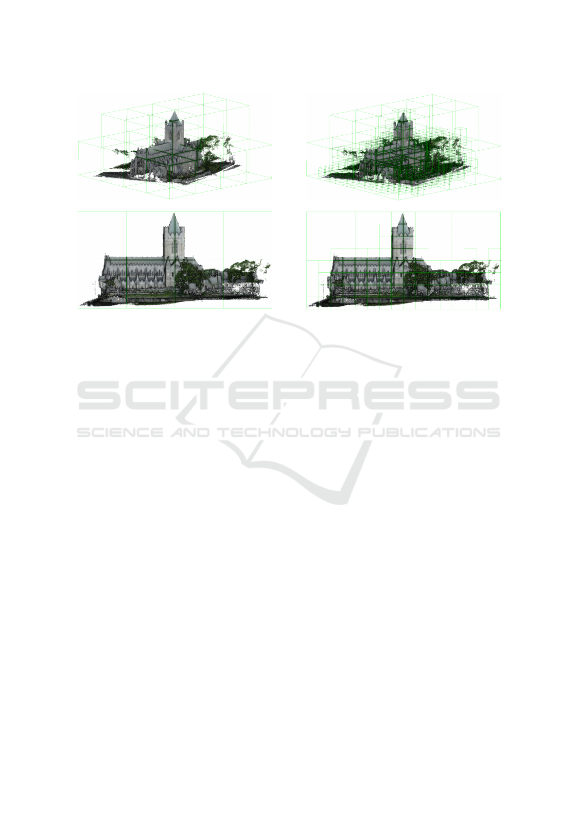
Figure 1: Tree depth one, the space is subdivided into 64

cells. The occupied cells are shown in green.

3 THE VOLA FORMAT

VOLA is unique in that it combines the beneﬁts of

partitioning algorithms with a minimal voxel format.

It hierarchically encodes 3D data using modular arith-

metic and bit counting operations applied to a bit ar-

ray. The simplicity of this approach means that it is

highly compact and can be run on hardware with sim-

ple instruction sets. The choice of a 64 bit integer as

the minimum unit of computation means that modern

processor operations are already optimized to handle

the format. While octree formats either need to be

fully dense to be serialized or require bespoke seri-

alization code for sparse data, the VOLA bit array is

immediately readable without header information.

VOLA is built on the concept of hierarchically

deﬁning occupied space using “one bit per voxel”

within a standard unsigned 64 bit integer. The one-

dimensional bit array that makes up the integer value

is mapped to three-dimensional space using modular

arithmetic. The bounding box containing the points

is divided into 64 cells. If there are points contained

within a cell the bit is then set to 1 otherwise it is set

to zero. The result of the ﬁrst division is shown in

Figure 1.

For the next level each occupied cell is assigned

an additional 64 bit integer and the space is further

subdivided into 64 cells. Any unoccupied cells on the

upper levels are ignored allowing each 64 bit integer

to only encode for occupied space. The bits are again

set based on occupancy and appended to the bit array.

Figure 2: Tree depth two. Each occupied cell is subdivided

into 64 smaller cells.

The number of integers in each level can be computed

by summing the number of occupied bits in the previ-

ous level. The resolution increases fourfold for each

additional level as shown in ﬁgure 2

The process is repeated with each level increasing

the resolution of the representation by four until a res-

olution suitable for the data is reached. This depends

on the resolution of the data itself. The traditional

approach used is to compute the average points per

meter of the dataset and use this to compute a suit-

able tree depth. One of the issues raised in this work

is that the non-uniform distribution of points makes

this a poor metric. A new approach that approximates

voxel neighborhood is found to more accurately re-

ﬂect the dataset is discussed in Section 7.

4 AERIAL LiDAR DATASETS

Real world data obtained from aerial LiDAR scans

is used in this work as it analogous to point cloud

data that would be obtained from an embedded sys-

tem used for 3D navigation, such as in a drone or a

self driving car. The four datasets examined in this

work are:

• The 2010 ARRA LiDAR Golden Gate Sur-

vey (san, )

• The 2013-2014 U.S. Geological Survey CMGP

LiDAR: Post Sandy (new, )

• The Montreal 2012 LiDAR Aerien Survey (mon,

VOLA: A Compact Volumetric Format for 3D Mapping and Embedded Systems

131

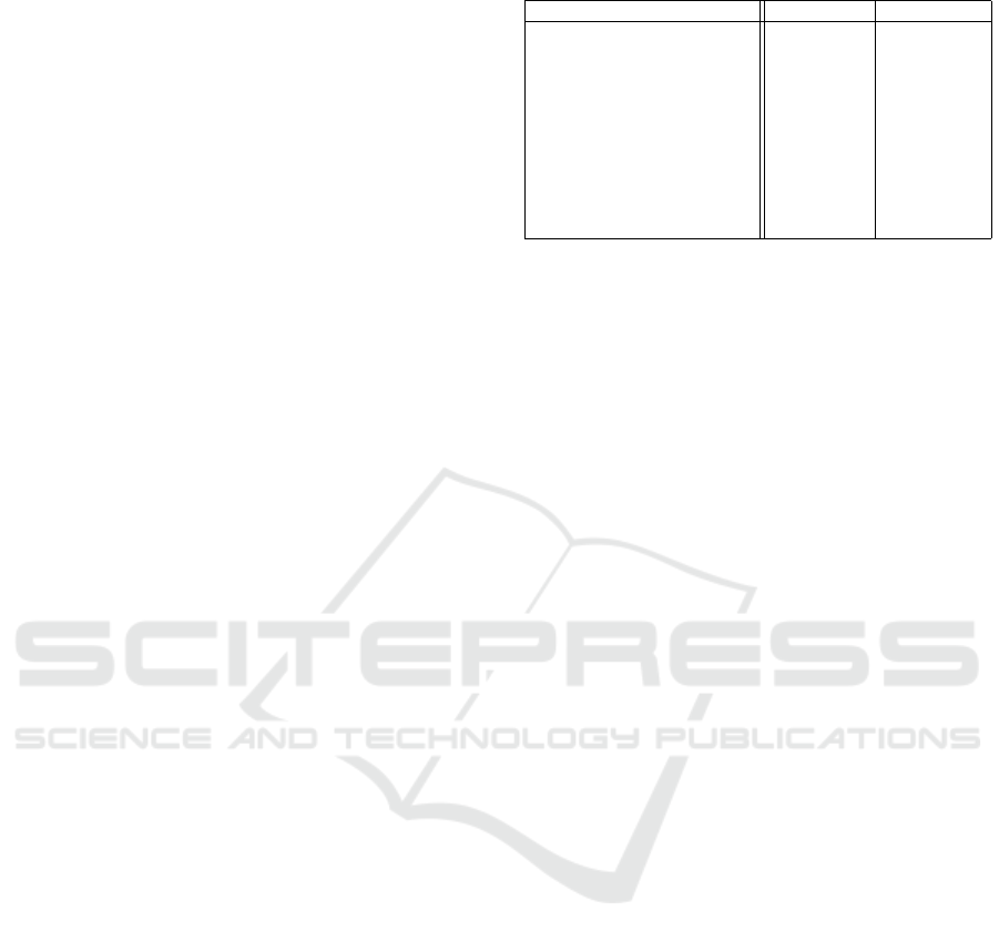
(a) Depth 1 (b) Depth 2

Figure 3: The output obtained for different tree depths. The

resolution increases by 4 for each axis on every successive

subdivision.

• The ALS 2015 Dublin survey (Laefer et al., )

The datasets were chosen as they model com-

plex built up urban environments and they are pub-

licly available open data (sﬂ, ; nyl, ; mon, b; dub,

). The density of the point clouds varies signiﬁcantly

between the datasets due to the ﬂight paths used to

gather the LiDAR data. Traditional GIS applications

are only concerned with generating Digital Elevation

Models which only requires a single height value per

grid point. Accordingly the amount of overlap be-

tween ﬂight paths was reduced to cover the maxi-

mum area in the least time and the resulting models

are sparse. The San Francisco, Montreal and New

York datasets followed this approach and so have a

low point density. The San Francisco dataset prov-

ing to be the sparsest at 0.2 points per meter, followed

by New York with 1.5 points per meter and Montreal

with 8 points per meter, as shown in Figures 4, 5,

and 6. The Dublin dataset was gathered by the Ur-

ban Modelling group which research techniques for

maximizing 3D data and model generation (Truong-

Hong et al., 2013). They used up to 60% overlap

in order to increase the point density to 190 points

per meter. The data was captured at an altitude of

300m using a TopEye system S/N 443. It consists

over 600 million points with an average point den-

sity of 348.43points/m

. It covered an area of 2km

in Dublin city center.

One issue that is obvious with the datasets is that

point distribution is not uniform. Aerial LiDAR scans

are inherently biased due to the angle and height at

which the data is gathered. This is clearly highlighted

in Figures 6and 7 where the roofs are bright green

Figure 4: San Francisco LiDAR scan density. The points

are uniformly distributed with an average density is 0.2

points per meter.

Figure 5: The New York LiDAR scan is uniform and of

higher density (1.5 points per meter) than the San Francisco

scan but is missing the facades on the buildings.

and red, representing a higher point density. There

are more point returns generated by higher ﬂatter sur-

faces, such as the roofs of buildings, rather than oc-

cluded street level structures. The average point den-

sity does not give an accurate representation of the un-

derlying data which is necessary for choosing the cor-

rect level of subdivision when voxelizing the dataset.

Our experiments show that the block occupancy,

which is analogous to a voxel neighborhood, gives a

more realistic metric of the point density by ﬁnding

the level of subdivision where the voxels become sep-

arated due to insufﬁcient point density. The metric

will be explained in more detail in the Section 7.

5 EXPERIMENTS

Two experiments are carried out in this work. The

ﬁrst experiment examines the difference between a

traditional dense mapping of the space using a 1

bit per voxel representation versus the hierarchical

GISTAM 2018 - 4th International Conference on Geographical Information Systems Theory, Applications and Management

132

Figure 6: The Montreal LiDAR scan density is 8 points per

meter and starts to show a non uniform distribution. The

rooftops and overlapping scan lines show up in green and

orange respectively.

Figure 7: The Dublin LiDAR scan density is 190 points

per meter and the distribution towards the rooftops is clearly

visible.

sparse mapping used by VOLA. The second exper-

iment compares standard and compressed VOLA to

the industry standard for point cloud compression, the

LAZ format.

5.1 Comparison of Dense Versus Sparse

Mapping

VOLA combines a 1 bit per voxel representation with

a hierarchical encoding. Rather than using 32 bit in-

teger to represent a voxel as in standard approaches,

the occupancy of each voxel is indicated by setting a

bit to 1. This encoding step alone will make the ﬁle

size 32 times smaller. What is unclear is the magni-

tude of reduction in ﬁle size results from a hierarchi-

cal compression. The worst case scenario, where the

points uniformly throughout the bounding box, would

result in dense and sparse volumes being of equal size.

The experiment measures the size reduction produced

by hierarchically encoding real world data. As both

Figure 8: Sparse versus Dense Encoding.

dense and sparse representations use one bit per voxel,

the one variable effecting ﬁle size is that the sparse

representation may omit empty space.

The sparse mapping discards any 64 blocks that

exclusively contain zeros. This means that empty

space is not encoded for but it adds an additional

overhead in processing time when packing and un-

packing the structure. Theoretically the worst case

for a sparse mapping, where points are uniformly

distributed throughout the space, would result in the

dense mapping and sparse mapping having equal size.

Fortunately points clouds based on real world data

generally have non-uniform distributions with most

point clouds consisting of empty space. (Klingen-

smith et al., 2015) found that only 7% of the space in

a typical indoor scene is in fact occupied. The density

of the Dublin LiDAR scan, for example, has an aver-

age occupancy of 1.36% per 100 meter tile. This work

examines the levels of compression obtained when

converting a point cloud to both dense and sparse rep-

resentations and how this is effected by the depth.

5.2 Comparison with LAS File Format

The VOLA format is compared to commonly used

industry standard for LiDAR data, the LAS ﬁle for-

mat. LAS is a binary format originally released by

the American Society of Photogrammetry and Re-

mote Sensing (ASPRS) for exchanging point cloud

data. LAS was designed as an alternative to propri-

etary formats or the commonly used generic ASCII

format. It has the ability to embed information on

the dataset and the points themselves, such as coordi-

nate reference system, number of returns, scan angle,

etc. An addition to this format is the compressed LAZ

format developed by (Isenburg, 2013). It is a lossless

format that takes advantage of the fact that LAS stores

the coordinates using a ﬁxed point format to compress

VOLA: A Compact Volumetric Format for 3D Mapping and Embedded Systems

133

the data. The resulting ﬁles are between 7% and 25%

of the original size. LAZ is now become the de facto

standard for point cloud formats.

The comparison with VOLA has two caveats:

ﬁrstly, converting a point cloud to a voxel format will

implicitly simplify the distribution to a binary grid

distribution. A voxel is placed in the grid if there is at

least 1 point in the grid location. A voxel could result

from a single point or 1000 points and so information

on high point concentrations is lost. The result is that

the conversion to a voxel format is lossy.

The second consideration is that the LiDAR for-

mat contains meta-data about the points themselves,

such as color, intensity, number of returns, scan angle,

etc. Using 1 bit per voxel VOLA means that only the

occupancy is recorded. In order to carry out a fairer

comparison, 2 Bits per voxel VOLA is used to rep-

resent the point meta-data. The meta-data is encoded

in byte blocks which means the resolution of the val-

ues is reduced from 32 bits to 8 bits but as much of

this data is normally limited to this range (intensity,

number of returns) then there is no loss of informa-

tion. There is data loss on the resolution of the data

as 2 bits per voxel records the information for a 64 bit

occupancy block rather than the individuals voxels.

In order to compare point cloud compression with

VOLA compression we used a standard compression

algorithm on the VOLA format. While VOLA is com-

pact it is not compressed and so there is still sig-

niﬁcant room for further ﬁle size reduction, whereas

the LAZ cannot be reduced further. The standard

gzip (Deutsch and Gailly, 1996) library was used to

compress the ﬁles. Gzip uses the deﬂate algorithm

for compression (Deutsch, 1996). The resolution of

the data used in this comparison was chosen by the

occupancy as calculated in the dense versus sparse ex-

periments. A resolution was chosen where the aver-

age block occupancy is above 15% which means that

there is a increased likelihood that the voxels are con-

nected.

6 DENSE VERSUS SPARSE

COMPARISON RESULTS

Each dataset was computed to multiple depths (and

therefore resolutions) in order to understand how the

ﬁle size compression was effected by the resolution.

The ﬁle size in megabytes was recorded for both the

dense and sparse representation. The improvement in

compression was computed by dividing the dense ﬁle

size by the sparse ﬁle size. An additional measure of

occupancy was computed by summing the bits in each

64 bit block in the sparse representation. This does

not give the actual neighborhood of a voxel, e.g., a

neighboring voxel could be contained in an adjoining

block, it does give an approximate measure of occu-

pancy.

The results for the San Francisco dataset are

shown in Table 2. Although this is the least dense

dataset it contains the largest number of tiles. The

magnitude reduction increases as the depth (and ac-

cordingly resolution) increases. The maximum com-

pression is 38 times smaller than the dense represen-

tation.

The initial occupancy is 46% at depth 1 which

then increases at depth 2 before decreasing again.

This is because the majority of bounding box is empty

space with most of the points having low height val-

ues.

It is also noted at depth 4 that the initial occupancy

of the voxel blocks falls below 10%. Each voxel in a

block can have up to 26 neighboring voxels of which

6 can be contiguous, i.e.,sharing a common face. As

the occupancy drops the likelihood of contiguity also

decreases. This is covered in more detail in Section 7.

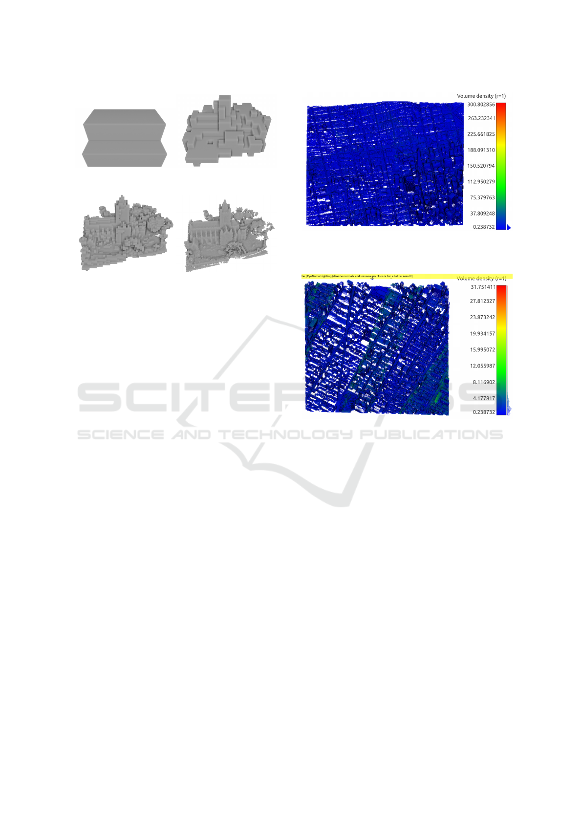
Table 2: Depth results for San Francisco dataset for 234887

tiles.

Lvl Dense(MB) Sparse(MB) Mag

Red

Block

Occup

1 1.87 1.87 1 46.77%

2 122.14 40.2 3.04 51.93%

3 7818.92 881.3 8.87 29.70%

4 500412.66 12918.8 38.74 7.3%

The New York dataset in Table 3 shows a similar

reduction in ﬁle size for increasing depth with a simi-

lar magnitude reduction for depth 4. There is also the

same increase in block occupancy at depth 2 before it

decreases and is less than 10% at depth 4.

Table 3: Depth results for New York dataset for 86804 tiles.

Lvl Dense(MB) Sparse(MB) Mag

Red

Block

Occup

1 0.694 0.694 1 39.15%

2 45.138 13.197 3.42 60.42%

3 2889.53 318.82 9.06 31.25%

4 184930.71 4858.55 38.06 9.62%

The Montreal dataset results in Table 4 shows a

slightly more pronounced reduction in ﬁle size ini-

tially but is only 34 times smaller by depth 4. The

occupancy again spikes at depth 2 and reaches 15% at

depth 4. This would imply that more detailed features

are captured in the higher resolution.

The Dublin dataset results are shown in Table 5.

Due to the signiﬁcantly higher point density it was

decided to increase the maximum depth to 5. This is

GISTAM 2018 - 4th International Conference on Geographical Information Systems Theory, Applications and Management

134

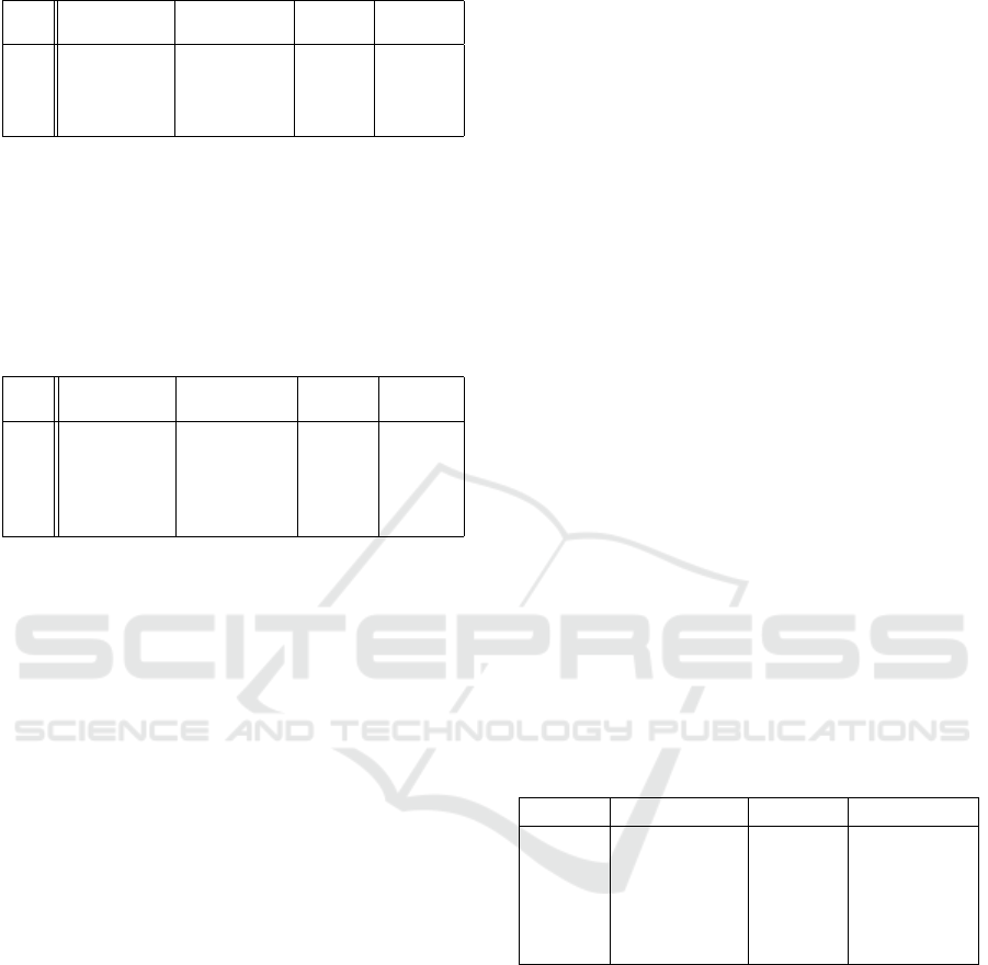
Table 4: Depth results for Montreal dataset for 66299 tiles.

Lvl Dense(MB) Sparse(MB) Mag

Red

Block

Occup

1 0.53 0.53 1 35.62%

2 34.47 9.44 3.65 62.52%

3 2206.96 233.08 9.47 37.97 %

4 141246.04 4106.08 34.4 15.62%

equivalent to each voxel representing a 9.7cm

cube

in the dataset. There is a smaller reduction in the ﬁle

size for successive depths compared to the previous

datasets but this increases to 70 time smaller at depth

5. The occupancy spikes at 87% at depth 2 and then

drops off to a minimum of 14.72%.

Table 5: Depth results for Dublin dataset for 356 tiles.

Lvl Dense(MB) Sparse(MB) Mag

Red

Block

Occup

1 0.0028 0.0028 1 52.5%

2 0.185 0.065 2.82 87.14%

3 11.85 1.96 6.05 48.33%

4 758.43 40.84 18.57 35.46%

5 48539.947 684.36 70.93 14.72%

6.1 Discussion

As stated earlier, if the data was distributed uniformly

throughout the bounding box this would result in

dense and sparse volumes being of equal size. The

experiments show that this is not the case with real

world data. There is an initial low occupancy for the

highest level encoding as the majority of points in

each 100m

tile are in the lowest third on the verti-

cal axis. Once this has been removed the remaining

space is largely occupied but then decreases for each

successive increase in resolution.

The magnitude of the reduction decreased for

more dense datasets but this was offset by a marked

increase in the magnitude of reduction for greater

depths. Although higher resolution datasets require

higher resolution VOLA models, increasing the res-

olution of sparse models increased the magnitude of

the space saving.

There was also a point with all the datasets where

the resolution increased to the point that the voxels

were no longer connected. The result is a voxel rep-

resentation where the number of voxels is the same as

the number of points (which is essentially a lossless

encoding of the data) but is not useful when comput-

ing collisions and navigation information. We shall

go into more detail on this in the next section.

7 BLOCK OCCUPANCY

Increasing the resolution resulted in greater number of

the points being disconnected. Although this means

that it more accurately represents the underlying point

cloud, it is less useful when using the representa-

tion for navigation or using machine learning on the

dataset. For example, analyzing a building facade or

detecting buildings using a 3D CNN require that the

data be connected into a contiguous object.

The true neighborhood of a voxel is difﬁcult to

compute when using a hierarchical encoding as it re-

quires ﬁnding neighboring blocks when a voxel is on

the edge of the current block. An alternative approach

is to conduct a bitwise comparison on the voxels or to

compute Euclidean distance between the voxels in a

block and ignore neighboring blocks. This simpliﬁes

the problem but it is still computationally expensive

due to the number of comparisons required.

A more efﬁcient although less accurate approach

is to compute the occupancy of a block, as was used

in the previous experiments. The occupancy of a 64

bit block is computed by summing the bits set to one.

This is not the true is only an approximation of neigh-

borhood but it does give a clear probability of the

connected components in a block. A comparison of

the occupancy and its relationship with the number

of connected components is shown in Table 6 and is

found to closely approximate to the number of con-

nections per block.

Table 6: A comparison of occupancy and the number of

connected voxels within a block.

Occup Contig Vox StdDev Connected

100% 144 0 100%

75% 80.44 3.23 55.8%

50% 35.31 3.38 24.5%

25% 8.58 2.28 5.9%

10% 1.49 1.09 0.75%

The point density is traditionally used when work-

ing out the suitable resolution for a voxelised model

but this approach oversimpliﬁes the distribution of the

data. It assumes the points have a uniform density

although the points tend to be biased towards areas

least occluded from the scanner, e.g., aerial LiDAR

data has many more times the points at the rooftops

than on ground level. It also takes no account for

the spread of points, i.e., points may cover a build-

ing consistently but only sparsely. Ignoring this worst

case resolution will result in fragmented voxel mod-

els. Although block occupancy may be an imperfect

metric, it is easy to compute and correlates well with

block contiguity. As such it provides a useful mecha-

VOLA: A Compact Volumetric Format for 3D Mapping and Embedded Systems

135

nism when determining what is a sufﬁcient resolution

when processing a dataset.

8 LAS FORMAT COMPARISON

RESULTS

The VOLA format is compared against the Laszip for-

mat using a two bits per voxel representation. This

allows for the meta-data about the points to be en-

coded. The caveats are that VOLA is not a lossless

format and the resolution of the point information is

reduced due to the hierarchical encoding. The point

information is averaged over each 64 bit block. There

is then a comparison against VOLA when compressed

using a gzip, a generic compression library. The depth

chosen for the data was based on the previous results

where the voxels are still connected. The San Fran-

cisco, New York and Montreal datasets are at depth 3

and the Dublin dataset is at depth 4. The VOLA for-

mat now allows for an arbitrary amount of additional

information to be appended to the structure, although

only 2 bits are used in this example.

Table 7: A comparison of the ﬁle size reduction when using

LAZ and VOLA.

Dataset LAS LAZ % VOLA % VOLAZip %

San Fran 224GB 33GB 14.7% 1.76GB 1.07% 799MB 0.35%

New York 126GB 22GB 17.4% 637MB 0.5% 336MB 0.26%

Montreal 167GB 27.7GB 16.5% 466MB 0.27% 189 0.11%

Dublin 36GB 3.7GB 10.27% 81.68MB 0.22% 33MB 0.091%

The results show that VOLA can reduce the ﬁle

size on the datasets to less than 1% their original size.

VOLA compressed using generic methods further re-

duces this by up to 50%. Although LAZ offers sig-

niﬁcant lossless compression, compressed VOLA re-

duces the ﬁle sizes to less than 5% of the LAZ ﬁles.

9 CONCLUSIONS

In this work we showed that encoding real-world data

using the hierarchical VOLA encoding massively re-

duces the ﬁle size. We also introduce a metric based

on voxel block occupancy that more accurately re-

ﬂects the underlying point cloud distribution than av-

erage point density. Although it is only an approxi-

mation of neighborhood it is easily calculated using

VOLA’s block format.

We then compared the VOLA representation with

point meta-data with standard LiDAR formats. The

reduction of the ﬁle size when compared with the

LAS format less than 1%, albeit at the loss of some

resolution and point information. Using a generic

compression algorithm on VOLA results in it being

5% of the ﬁle size of the compressed LAZ format.

Due to the inherent sparsity of real-world data, a

hierarchical encoding that omits empty space makes

sense. These results show that it is possible to store

large amounts of 3D data in a memory footprint that

could easily be accommodated on an embedded sys-

tem for both mapping and machine learning applica-

tions.

10 FUTURE WORK

A generic compression algorithm was used to com-

press the data. This could be improved using bespoke

techniques developed for the underlying 3D data such

as run length encoding and look up tables for self sim-

ilar features. Our intention is to use such techniques

to further reduce the ﬁle size.

REFERENCES

The 2010 arra lidar: The golden gate lidar project.

https://data.noaa.gov/dataset/2010-arra-lidar/-golden-

gate-ca. Accessed: 2017-10-05.

2013-2014 u.s. geological survey cmgp lidar: Post sandy

(new york city). https://data.noaa.gov/dataset/2014-

u-s-geological-survey/-cmgp-lidar-post-sandy-new-

jersey. Accessed: 2017-10-05.

Dublin als2015 lidar license (cc-by 4.0).

https://geo.nyu.edu/catalog/nyu 2451 38684. Ac-

cessed: 2017-10-19.

Montreal lidar aerien 2015.

http://donnees.ville.montreal.qc.ca/dataset/lidar-

aerien-2015. Accessed: 2017-10-05.

Montreal lidar license (cc-by 4.0).

http://donnees.ville.montreal.qc.ca/dataset/lidar-

aerien-2015. Accessed: 2017-10-19.

Post sandy lidar survey license.

https://data.noaa.gov/dataset/2014-u-s-geological-

survey-cmgp/-lidar-post-sandy-new-jersey. Ac-

cessed: 2017-10-19.

San francisco arra lidar license.

https://data.noaa.gov/dataset/2010-arra-lidar-golden-

gate-ca. Accessed: 2017-10-19.

Bentley, J. L. (1975). Multidimensional binary search trees

used for associative searching. Communications of the

ACM, 18(9):509–517.

Boissonnat, J.-D. (1984). Geometric structures for three-

dimensional shape representation. ACM Transactions

on Graphics (TOG), 3(4):266–286.

Crassin, C., Neyret, F., Lefebvre, S., and Eisemann, E.

(2009). Gigavoxels: Ray-guided streaming for efﬁ-

cient and detailed voxel rendering. In Proceedings of

the 2009 symposium on Interactive 3D graphics and

games, pages 15–22. ACM.

GISTAM 2018 - 4th International Conference on Geographical Information Systems Theory, Applications and Management

136

Deutsch, P. (1996). Deﬂate compressed data format speci-

ﬁcation version 1.3.

Deutsch, P. and Gailly, J.-L. (1996). Zlib compressed data

format speciﬁcation version 3.3.

Geosystems, L. (2015). Leica scanstation p30/p40. Product

Speciﬁcations: Heerbrugg, Switzerland.

Girardeau-Montaut, D. (2006). Change detection on three-

dimensional geometric data. PhD thesis, T e l e com

ParisTech.

Hornung, A., Wurm, K. M., Bennewitz, M., Stachniss, C.,

and Burgard, W. (2013). Octomap: An efﬁcient prob-

abilistic 3d mapping framework based on octrees. Au-

tonomous Robots, 34(3):189–206.

Hughes, J. F., Van Dam, A., Foley, J. D., and Feiner, S. K.

(2014). Computer graphics: principles and practice.

Pearson Education.

Isenburg, M. (2013). Laszip. Photogrammetric Engineering

& Remote Sensing, 79(2):209–217.

Kazhdan, M., Bolitho, M., and Hoppe, H. (2006). Poisson

surface reconstruction. In Proceedings of the Fourth

Eurographics Symposium on Geometry Processing,

SGP ’06, pages 61–70, Aire-la-Ville, Switzerland,

Switzerland. Eurographics Association.

Klingensmith, M., Dryanovski, I., Srinivasa, S., and Xiao,

J. (2015). Chisel: Real time large scale 3d reconstruc-

tion onboard a mobile device using spatially hashed

signed distance ﬁelds. In Robotics: Science and Sys-

tems, volume 4.

Laefer, D. F., Abuwarda, S., Vo, A.-V., Truong-Hong,

L., and Gharibi, H. 2015 aerial laser and pho-

togrammetry survey of dublin city collection record.

https://geo.nyu.edu/catalog/nyu 2451 38684. Ac-

cessed: 2017-10-05.

Laine, S. and Karras, T. (2011). Efﬁcient sparse voxel oc-

trees. IEEE Transactions on Visualization and Com-

puter Graphics, 17(8):1048–1059.

Meagher, D. (1982). Geometric modeling using octree en-

coding. Computer graphics and image processing,

19(2):129–147.

Mutto, C. D., Zanuttigh, P., and Cortelazzo, G. M. (2012).

Time-of-ﬂight cameras and microsoft kinect (TM).

Springer Publishing Company, Incorporated.

Nardi, L., Bodin, B., Zia, M. Z., Mawer, J., Nisbet, A.,

Kelly, P. H. J., Davison, A. J., Luj

an, M., O’Boyle,

M. F. P., Riley, G., Topham, N., and Furber, S.

(2015). Introducing SLAMBench, a performance and

accuracy benchmarking methodology for SLAM. In

IEEE Intl. Conf. on Robotics and Automation (ICRA).

arXiv:1410.2167.

Peucker, T. K., Fowler, R. J., Little, J. J., and Mark, D. M.

(1978). The triangulated irregular network. In Amer.

Soc. Photogrammetry Proc. Digital Terrain Models

Symposium, volume 516, page 532.

Riegler, G., Ulusoys, A. O., and Geiger, A. (2016). Octnet:

Learning deep 3d representations at high resolutions.

arXiv preprint arXiv:1611.05009.

Truong-Hong, L., Laefer, D. F., Hinks, T., and Carr, H.

(2013). Combining an angle criterion with voxeliza-

tion and the ﬂying voxel method in reconstructing

building models from lidar data. Computer-Aided

Civil and Infrastructure Engineering, 28(2):112–129.

VOLA: A Compact Volumetric Format for 3D Mapping and Embedded Systems

137