Towards a Knowledge-driven Maintenance Support System for

Manufacturing Lines

E. Garcia

, N. Montes

and M. Alacreu

Ford Spain, Pol

ıgono Industrial Ford S/N, CP 46440, Almussafes, Valencia, Spain

Department of Mathematics, Physics and Technological Sciences, University CEU Cardenal Herrera, C/ San Bartolom,

55, Alfara del Patriarca, Valencia, Spain

Keywords:

Knowledge-driven Support System, Maintenance, Prognosis, Mini-term, Change Point.

Abstract:

This paper presents how to design a Knowledge-driven Maintenance Support System (MSS) to prognostic

breakdowns in production lines and how it affects to the production rate. The system is based on the sub-

cycle time monitorization and how the cycle time variability of machine parts can be used as a deterioration

indicator that could describe the dynamic of the failure for the machine parts. For this proposal, a novel model

based on mini-terms and micro-terms introduced in our previous work as a machine subdivision is used. A

mini-term subdivision can be selected by the expert team for several reasons, the replacement of a machine

part or simply to analyze the machine more adequately. (A micro-term is a component from a mini-term and

it can be as small as the user wishes. Without loss of generality, the paper focuses its attention on a welding

line at Ford Motor Company located at Almusafes (Valencia) where a welding unit was isolated and tested

for some particular pathologies. The cycle time of each mini-term is measured by changing the deteriorated

components in the cycle time. The deterioration of the parts (a proportional valve, a cylinder, an electrical

transformer, the robot speed and the loss of pressure) are tested within the range of normal production, which

is the range that cannot be detected by alarms or maintenance workers but when the change point is occured.

The statistical analysis of the data obtained in the experiments allows us to deﬁne the rules that govern the

decisions for the real-time Knowledge-driven MSS. This analysis and the welding line simulation also allows

us to know the loss of productivity when the change point occurs. In the worst case, the welding line reduces

their production rate almost 40%.

1 INTRODUCTION

A production line is composed of a set of sequential

operations established in a factory whereby materials

are put through a reﬁning process to produce an end-

product.

During the lifespan of the line, which could be de-

cades, the throughput depends on an amount of pa-

rameters like, maintenance policy, downtime events,

machine breakdowns, deteriorating systems, dynamic

bottleneck behavior, bowl phenomenon, market de-

mand, etc. There are open questions to be resol-

ved that are not treated in literature in depth which

produces an enormous gap between academic the-

ory and real plant problems, bringing up a conside-

rable amount of research topics where maintenance

and replacement problems of deteriorating systems

are some of them.

Maintenance operations have a direct inﬂuence on

production performance in manufacturing systems.

Maintenance task prioritization is crucial and impor-

tant, especially when availability of maintenance re-

sources is limited. Generally, maintenance can be ca-

tegorized into two major classes: corrective mainte-

nance (CM) and preventative maintenance (PM). CM

is performed when a machine fails. It usually involves

replacing or repairing the component that is responsi-

ble for the failure of the overall system. However, PM

is performed before machine failure. The objective of

PM is to achieve continuous system production. In

condition-based maintenance framework, a deteriora-

tion indicator that correctly describes the dynamic of

the failure process is required. Usually, this efﬁcient

indicator can be constructed from collected informa-

tion on various deterioration-related monitoring pa-

rameters such as vibration, temperature, noise levels,

etc. However, the need of continuous monitoring may

increase the system costs when expensive monitoring

devices are required (A.K.S.Jardine and D.Banjevic,

2006). In fact, that is the main drawback in PM using

Garcia, E., Montes, N. and Alacreu, M.

Towards a Knowledge-driven Maintenance Support System for Manufacturing Lines.

DOI: 10.5220/0006834800430054

In Proceedings of the 15th International Conference on Informatics in Control, Automation and Robotics (ICINCO 2018) - Volume 1, pages 43-54

ISBN: 978-989-758-321-6

these techniques.

Over the last two decades, numerous prognos-

tic approaches have been developed. Prognostic is

a major scientiﬁc challenge for industrial implemen-

tation of maintenance strategies in which the remai-

ning useful life estimation (RUL) is an important task.

For environmental, economic and operational purpo-

ses, the prognostic and the remaining useful lifetime

prediction arouse a big interest. In the framework

of prognostic and health management (PHM), many

prognostic techniques exist and they are basically

classiﬁed into three principal classes: data-driven ap-

proaches, model-based approaches, experience-based

approaches, but these can also be classiﬁed in two

groups, non-probabilistic methods and probabilistic

methods, see (K.L.Son, 2013). In non-probabilistic

methods the deterioration phenomenon is not random

and in most observations the deterioration can be

fuzzy. With probabilistic methods, the deterioration

phenomenon is considered to be random and with sto-

chastic tools it is considered a random behavior. In

this case the prognostic is based on the future beha-

vior of the stochastic deterioration process and can

give results in terms of probabilities, see (K.L.Son,

2013).

1.1 Knowledge-driven Support Systems

and the Industry 4.0

In modern manufacturing, real-time control of pro-

duction operation to improve system responsiveness,

increase system efﬁciency and reduce downtime is be-

coming more and more critical. More recently, this

concept is moving forward to the concept of ”Industry

4.0”. It is a current trend and data exchange in ma-

nufacturing technologies. It includes cyber-physical

systems, the internet of things and cloud computing

creating what has been called a ”smart factory”. Most

manufacturing industries have sought to improve a

productivity and quality with this new techniques

where data-driven decision support systems (DSS)

appear as a new paradigm. In (S.H.Muhammad,

2017) we can ﬁnd a recent review on the use of DSS

in manufacturing. One of the data-driven DSS is the

one called Knowledge-driven DSS. It has its origin in

the Intelligent Decision Support Systems or in a broa-

der sense, in Artiﬁcial intelligence (AI),(H.R.Nemati,

2002) ,(M.Negnevitsky, 2005) . Knowledge-driven

DSS are computed-based reasoning systems with the

distinction that AI technologies, management expert

systems, data mining technologies and communica-

tion mechanism are integrated. Intelligent DSS are

divided in some evolutionary developments. One of

them is about rule-based expert systems (A.Chakir,

2016). These systems are based on the use of heuris-

tics, which can be understood as strategies that lead

to the correct solution for the problem. For this sys-

tems it is always necessary to use human expert kno-

wledge collected in a database, (M.Chergui, 2016).

Knowledge-driven DSS are successfully applied for

many applications like for instance, market manage-

ment, (M.Murthadha, 2013) or for radiation therapy

treatment planning (R.R.Deshpande, 2016).

The present study proposes a novel protocol on

how to design Knowledge-driven Maintenance Sup-

port Systems (MSS). Based on real-time measure-

ment of sub-cycle times, with the help of expert kno-

wledge and the statistical analysis of the measure-

ments, we could deﬁne rules that allow us to predict

the deterioration of a particular machine part or com-

ponent. In adition to that and, based on the same sta-

tistical analysis and the numerical simulation techni-

ques, allows us to know the loss of production produ-

ced by the component deterioration.

The present paper is organized as follows. Section

2 describes our previous works, in particular, the mat-

hematical model that will allow us to study sub-cycle

times,(E.Garcia, 2016), (E.Garcia and N.Montes,

2017).

Section 3 desribes the change point concept and

their link with the sub-cycle time.

Section 4 shows the experimental platform used to

design our Knowledge-driven MSS. This platform is

based on a welding unit used at Ford Motor Company

located at Almusafes (Valencia).

Section 5 describes the statistical analysis used to

deﬁne the rules of our Knowledge-driven MSS.

Section 6 describes the numerical simulation de-

veloped to compute the loss of production rate when

the change point occurs in a welding station.

Section 7 presents the conclusions with an empha-

sis on future research challenges towards a real-time

Preventive Maintenance Schedule System.

2 PREVIOUS WORK. FROM

MICRO-TERM TO

LONG-TERM

The data used in the analysis of the production lines

is classiﬁed into long-term and short-term. Long-term

is mainly used for process planning, while short-term

focuses, primarily, on process control. Following the

deﬁnition in (L.Li and J.Ni., 2009), short-term is re-

ferred to an operational period not large enough for

machine failure period to be described by a statis-

tic distribution. The machine cycle time is conside-

ICINCO 2018 - 15th International Conference on Informatics in Control, Automation and Robotics

Figure 1: Real change points measured in Ford Almussafes Factory.

Figure 2: A pyramid of terms.

red short-term. In (E.Garcia, 2016), (E.Garcia and

N.Montes, 2017) redeﬁnes short-term into two new

terms, mini-term and micro-term, see ﬁgure 2. A

mini-term could be deﬁned as a machine part, in a

predictive maintenance policy or in a breakdown, re-

placeable easier and faster than another machine part

subdivision. Furthermore, a mini-term could be deﬁ-

ned as a subdivision that allows us to understand and

study the machine behavior. These sub-cycle times

(micro-terms and mini-terms) are not the same at each

repetition and they follow a probabilistic distribution,

mean value µ and standard deviation σ. In addition to

that, the probabilistic sub-cycle time for each machine

component varies during the lifespan of the compo-

nent. In other words, the deterioration indicators that

can be measured with thermal cameras, vibration and

ultrasonic devices have an effect on the machine cycle

time. In most cases, the measurement of these cycle

times does not imply any additional costs because the

actuators that allow the sub-cycle time measurement

were installed in the machine and are used for their

automated work.

3 Mini-term DEGRADATION

PATH. A CHANGE POINT

Prediction and analysis of degradation paths are im-

portant to condition-based maintenance (CBM). It is

well known that the degradation paths are non-linear.

It means that in the degradation path, a sudden change

point apears when the RUL (Remaining Useful Life)

is near to the end, see (X.Zhao, 2018), (X.Zhao,

2014). Before the change point, the component works

in optimal conditions and after the change point the

component works in bad conditions anouncing that

the failure is near, see Figure 3.

Figure 3: Change point.

The change point in the physical part of the

machine components produce similar effect in the

sub-cycle time, that is a change point in the mini-

term, Figure 1 shows two examples measured at Ford

Almussafes factory. The ﬁrst one is a change point

produced in the mini-term due to the deterioration of

a welding clamp proportional valve. The second one

is a ciylinder with inner leakage, also in a welding

clamp. These change points in the mini-terms can

be detected using common data analysis techniques,

see (X.Zhao, 2018), (X.Zhao, 2014). When a change

point in the min-iterm is detected, an alarm must

Towards a Knowledge-driven Maintenance Support System for Manufacturing Lines

be activated for the maintenance workers in order

to replace it, as soon as possible. There are some

questions to solve about the use of mini-terms in

maintenance systems;

- Which kind of pathology produced the change

point?

- How it affects to the production rate?

- How many time have the maintenance worker to

replace it before breakdown?

The present paper treats to answer the ﬁrst two

questions.

4 WELDING LINE CASE

In order to test and illustrate the analysis of the pre-

sent paper, a real welding line located at Ford Al-

mussafes (Valencia) is used, see Figure 4. In a real

welding line like this, there are welding workstations

where, each one has welding stations working in pa-

rallel and sometimes in serial. Each welding station

makes some welding points in the same cycle time. It

is possible to ﬁnd 1,2,4 or at least 6 welding station

in the same workstation, where each one makes up to

19 welding points. In our particular case, our wel-

ding line has 8 workstations where workstation 1,5

and 6 have 4 welding units,workstations 2,4,7 and 8

have 6 welding stations and workstation 3 has 1 wel-

ding unit, see Figure 5. The welding line was instal-

led in 1980. The staff group that designed the line

deﬁned the maximum running capacity, ECR (engi-

neering running capacity), 60 JPH (Jobs Per Hour).

However, the plant engineers have another maximum

running capacity, that is the ERR (engineering run-

ning rate), in this case deﬁned in 51 JPH. Nowadays,

this line welds 68 different models and variants. Dif-

ferent car models with 3,5 doors with or without so-

lar roof, etc. Obviously, from 1980 to today, the line

suffers a lot of changes and updates, new models and

variants are appear and old models and variants disap-

peared, most advanced robot arms and welding units

are introduced, etc. Therefore, the line is re-balanced,

if it is possible, when new update occurs.

4.1 A Test Bench for a Welding Station

Without loss of generality, the present paper uses a

real welding station for Ford S.L. located at the Al-

mussafes factory as an example for the proposed met-

hodology. The welding station is one of the most re-

levant stations because there are 4,500 welding points

in a car. A robot arm and a welding clamp compose a

welding station, see ﬁgure 6. The behavior of the wel-

Figure 4: Welding line at Ford Almussafes (Valencia).

ding station is simple. First, the robot arm moves the

welding clamp to the point to weld. Then, a pneuma-

tic cylinder moves the welding clamp in two phases:

One to bring closer the clamp and a second one to

weld. The pressure applied by the clamp is controlled

by a control system.

The Robot Arm and Welding Clamp need a cer-

tain time to develop their task and their components

also need a certain time to develop their own tasks.

In order to analyze the deterioration effect of some

mini-terms, an expert team decided that the most con-

venient division is in three mini-terms, the robot arm,

the welding clamp motion and the welding task. The

reason was that it is easier and faster to replace these

parts in a maintenance tasks than another machine

part subdivision.

Figure 7 shows the experimental setup to measure

the cycle time of each mini-term in the welding sta-

tion where the PLC and the PC are used to measure

the time. The experimental test is quite simple. The

robot arm, starting from a predeﬁned initial point, mo-

ves the clamp to a predeﬁned welding point; then the

clamp is closed and develops the welding task.

4.2 Pathologies Analysed

The welding station, as well as other stations in the

industry, is bound to suffer from pathologies that pro-

duce an effect on the cycle time. Based on the opera-

tor’s experience, we selected the most common ones

for the experimental welding station. These patho-

logies produce a cycle time modiﬁcation but do not

produce failure of the component, going unnoticed for

maintenance workers and also for the control system,

in other words, after the change point and before the

failure of the component, see Figure 3. The patholo-

gies rated are; for the welding clamp mini-term: the

proportional valve, the cylinder stiffness, welding fai-

lure produced by the transformer and pressure loss,

and for the robot arm mini-term; the robot arm speed.

A brief description of each one is hereby explained:

ICINCO 2018 - 15th International Conference on Informatics in Control, Automation and Robotics

Figure 5: Welding line layout.

Figure 6: Welding station.

Figure 7: Experimental setup.

- Pathology 1 (P

) (Proportional valve): This valve

transmits the pressure to the cylinder and is managed

by the controller. It is responsible for maintaining the

proper pressure in the cylinder. During its lifetime, its

components suffer fatigues that produce the stiffness

of some of them. This condition creates a time delay.

When it is too deteriorated the valve cannot transmit

enough pressure to the cylinder and the welding task

is not possible.

- Pathology 2 (P

) (Cylinder stiffness): A critical

term in welding task is the pressure applied on the me-

tals. This force is necessary to ensure good electrical

contact between the parts to be welded, and to main-

tain the ﬁxed parts until the metal forming the solid

board has time to solidify. The elements responsible

for transmitting the proper pressure to these plates are

the cylinder clamps. If one of the cylinders has is

worn off, has galling or there is communication in-

side the stem, a time delay is produced. Maintenance

workers detect this pathology when the cylinder can-

not transmit enough pressure on the metals and the

welding task cannot be performed.

-Pathology 3 (P

) (Welding failure): The welding

process between parts consists of passing an electric

current through intensive metals in order to be joined.

The device generally used for this task is a transfor-

mer. The fatigue of this component is mainly pro-

duced due to the loss of wire insulation. It produces

a modiﬁcation in the value of the insulated resistance

and therefore produces a current reduction that affects

the welding time. Maintenance workers detect this

pathology when the welding task cannot be perfor-

med due to failure.

- Pathology 4 (P

) (Pressure loss): One of the most

common delays is produced by pressure losses in a

pneumatic circuit. The pressure drop causes a delay

or malfunction in the pneumatic devices to be opera-

ted. This pathology could be produced by many facts

such as a simple pore that produces a failure in the

compressor. Maintenance workers detect this failure

when the low pressure alarm is triggered.

- Pathology 5 (P

) (Robot Speed): The common

industrial robots have 6 axes. All these axes are syn-

chronized to achieve the points that have been deﬁned

by the program to perform its function or task. If there

is a failure in the operation, it causes an engine speed

reduction that directly affects the process cycle time.

There are several reasons that produce this pathology.

In these industrial robot arms, high speed and high

accurate operation are required. However, in the case

Towards a Knowledge-driven Maintenance Support System for Manufacturing Lines

of high speed operations, strong jerks often arouse,

i.e., rapid change of acceleration. Jerk causes deterio-

ration of control performance such as vibration in a tip

of a robot arm. Jerk forces are not equally distributed

and as the robot arm does the same movement again

and again, the deterioration is located in some parti-

cular joint. Mechanical structure deterioration or the

deterioration of electrical parts also affects the speed.

This pathology is very difﬁcult to detect by mainte-

nance workers because it does not produce the break-

down of the machine and, as the robot moves at high

speed, it is nearly impossible to be detected without a

speciﬁc procedure.

4.3 Experimental Test

The experimental methodology is as follows. The

clamping task is to weld the same point 6 times in

order to obtain enough time precision. The robot arm

trajectory is the same in all the movements. Then, the

clamping task is repeated 40 times in order to obtain

a sufﬁcient number of samples to measure the mean

value and the standard deviation for each mini-term.

As the welding motion and the welding task are low

time consuming, the task is repeated 6 times to obtain

one of the forty samples. Firstly, the welding clamp

station is tested without the hereby explained patho-

logies. Secondly, a particular component with each

pathology is replaced in the station and the test is re-

peated.

5 RULES DEFINITION BASED ON

STATISTICAL ANALYSIS

The goal of the present section is to analyze the expe-

rimental samples to understand how the pathologies

affect the cycle time and to generate rules that allow

us to deﬁne our Knowledge-driven MSS. From now

on, we are going to call Control, without pathology,

as ”C” and the behaviour with one of the pathologies

...P

), that is, six different situations for each mini-

term. There are 40 samples for each situation, that is

n = 240 for each miniterm. As the times for the wel-

ding clamp motion and for the welding clamp task

mini-term are obtained repeating the task six times,

each sample is precomputed as;

(1)

where x

is the i

sample obtained by the z

sample

that contains 6 repetitions.

The statistical tests used in the present section are

Shaphiro-Wilk, Levene, ANOVA, Kruskal-Wallis and

a variance. For all the tests, the signiﬁcance level is

α = 0.05. After the descriptive analysis of the data,

see Figure 8, it is obvious that the cycle time for

the mini-terms with pathology are different compared

with the control or bassal situation. Next subsections

analyze, in detail, each mini-term.

5.1 Robot Motion mini-term Analysis

Table 1: Robot motion mini-term.

n Shapiro −Wilk Variance Mean;Sd

P −Value

C 40 0.8186 0.0005 35.5497;0.0215

40 0.2150 0.0011 35.5472;0.0336

40 0.7667 0.0007 35.5496;0.0257

40 0.7671 0.0013 35.5492;0.0361

40 0.5451 0.0009 35.5485;0.0302

40 0.0559 0.0010 46.3314;0.0314

Levene ANOVA

P − value P − value

= 0.0824 < 0.0001

5.1.1 Normality Analysis

Shapiro-Wilk test is used to analyze if the groups fol-

low a normal distribution. Table 1 shows the p-values,

where all of them are meaningful, meaning that each

group, independently of the pathology, is able to be

approximated to a normal distribution.

5.1.2 Homogeneity of Variances

Levene test is used to analyze if there are differences

among variances for the control group and patholo-

gies. As can we see in Table 1, p-values are meaning-

ful meaning that there are no signiﬁcant differences

among them.

5.1.3 Mean Analysis

After to check that the groups follow a normal distri-

bution and the variances have no signiﬁcant differen-

ces, ANOVA test can be computed, see Table 1. The

conclusion is that at least two of the six situations are

signiﬁcativaly different. Tukey’s range test allow us to

check this result as well as to determine which mean

values are different and to sort them, see Figure 9

Therefore, the rule obtained for the mean value is:

= µ

< µ

(2)

It means that there are no signiﬁcant differences

among the mean value without pathology and the

mean time for pathologies P

, P

. However

ICINCO 2018 - 15th International Conference on Informatics in Control, Automation and Robotics

Figure 8: Descriptive analysis.

Figure 9: Tukey test for the robot motion miniterm.

there are signiﬁcant diferences with P

and can be de-

tected by means of the robot motion mini-term.

5.1.4 Variance Analysis

Although with the Levene test it is possible to con-

clude that there are no signiﬁcant differences among

variances, for practical purposes, it is observed that

when a pathology exists, the standard deviation also

increases, see Table 1. Therefore, it is possible to

deﬁne a contrast hypothesis individually through the

basal variance (0.0005) for each one of the patholo-

gies (σ

> σ

), distributed as a Chi-Squared,

n−1

to estimate the standard deviation limit that, up to it,

detects a pathology. As a result, if the standard devia-

tion is greater than 0.0254, a pathology is expected.

5.2 Welding Clamp Motion mini-term

Analysis

Table 2: Welding clamp motion mini-term.

n Shapiro −Wilk Variance Mean;Sd

P −Value

C 40 0.5069 0.0000 0.4158;0.0061

40 0.5727 0.0000 0.4302;0.0060

40 0.0542 0.0002 1.4087;0.0448

40 0.0869 0.0000 0.4643;0.0070

40 0.0040 0.0024 1.5594;0.0489

40 0.7584 0.0000 0.4185;0.0060

Levene

C, P

1−5

P − value

< 0.0001

Levene ANOVA

C, P

1,3,5

C, P

1,3,5

P − value P − value

< 0.7538 < 0.0001

Levene Kruskal −Wallis

2,4

P − value P − value

< 0.0001 < 0.0001

5.2.1 Normality Analysis

Shapiro-Wilk test is used to analyze if the groups have

a normal distribution. As can we see in Table 2, p-

values are meaningful except for P

. It means that

it is possible to detect pathology 4 by means of this

criteria.

5.2.2 Homogeneity of Variances

Levene test is used to analyze if there are differences

among variances for the control group and patholo-

gies. As can we see in Table 2, there are no signiﬁcant

differences for the group {C, P

, P

}. However, cy-

cle times for the group {P

, P

} do not accomplish this

criteria.

Towards a Knowledge-driven Maintenance Support System for Manufacturing Lines

5.2.3 Mean Value Analysis

After to check if the groups have a normal distribu-

tion and if there are signiﬁcant differences among

variances, ANOVA test is computed just for the

groups that accomplish the applicability criteria, that

is, {C,P

, P

}, see Table 2. The conclusion is that

at least two of the four situations are signiﬁcativaly

different. Tukey’s range test allow us to check this

result as well as to determine which mean values are

different, see Figure 10.

Figure 10: Tukey test for the clamp motion miniterm.

By means of the Tukey’s range test it is possible

to obtain the next rule;

= µ

< µ

(3)

The other two pathologies, P

and P

are analyzed

using Kruskal- Wallis, see Table 2. As a conclusion,

pathology P

is signiﬁcantly greater than Pathology

. Therefore, mean rule for the welding motion mini-

term is;

= µ

< µ

(4)

5.2.4 Variance Analysis

As can we see at the Levene test, all the groups do not

accomplish homogeneity of variances. However, as in

the robot motion variance analysis, it is observed that

when a pathology exists, the standard deviation also

increases, see Table 2. This fact has a direct relati-

onship with the change point if basal sample variance

is considered as a population sample variance (σ

Therefore, using a contrast hypothesis, σ

6= σ

, dis-

tributed as a Chi-Squared,

n−1

, it is possible to esti-

mate the standard deviation that detect pathologies P

and P

, that is S

6∈ [0.0048, 0.0075].

Therefore, the rule obtained for the welding clamp

motion variance values is:

= σ

< σ

(5)

5.3 Welding Clamp Task mini-term

Analysis

Table 3: Welding clamp task mini-term

n Shapiro −Wilk Variance Mean;Sd

P −Value

C 40 0.9905 0.0001 1.4373;0.0109

40 0.0102 0.0251 4.0523;0.1585

40 0.4012 0.0061 1.1391;0.0783

40 0.8340 0.0001 1.4389;0.0119

40 0.2287 0.0044 1.2945;0.0665

40 0.1851 0.0001 1.4489;0.0110

Levene

C, P

1−5

P − value

< 0.0001

Levene ANOVA

C, P

3,5

C, P

3,5

P − value P −value

= 0.788 < 0.0001

Levene ANOVA

2,4

P − value P −value

= 0.3105 < 0.0001

5.3.1 Normality Analysis

Shapiro-Wilk test is used to analyze if the groups have

a normal distribution. As can we see in Table 3, p-

values are meaningful except for P

. Therefore, it is

possible to detect P

by means of this criteria.

5.3.2 Homogeneity of Variances

Levene test is used to analyze if there are differen-

ces among variances for the control group and patho-

logies. As can we see in Table 2, there are signiﬁ-

cant differences among {C, P

, P

}. Howe-

ver, following the descriptive analysis depicted in Fi-

gure 8, the analysis is repeated splitting the groups in

two groups, G

= {C,P

, P

} and G

= {P

, P

}. As

can we see in Table 3, Levene test is accomplished in

both cases.

5.3.3 Mean Value Analysis

Following the same steps of the previous subsection,

ANOVA test is applied following the same group di-

ICINCO 2018 - 15th International Conference on Informatics in Control, Automation and Robotics

Table 4: Rules for the Knowledge-driven MSS. Welding station case.

mini-term mean rules variance rules Stand. desv. rules normality rule

Robot Motion µ

= µ

< µ

− − − S > 25.4 · 10

−3

→ All − − −−

Welding Motion µ

= µ

< µ

= σ

< σ

S 6∈ [47 · 10

−4

74 · 10

−4

] → P

, P

P4 f ail

Welding task µ

< µ

= µ

< µ

= σ

< σ

= σ

< σ

S > 12.9 · 10

−3

→ P

, P

P1 f ail

vision, see Table 3. For both groups G

, G

, the con-

clusion is that at least two situations are signiﬁcativaly

different. Figure 11 and ﬁgure 12 show the Tukey test

result.

Figure 11: Tukey test for the clamp task mini-term, G

Figure 12: Tukey test for the clamp task mini-term, G

Therefore, the rule obtained for the welding clamp

motion mean values is:

< µ

= µ

< µ

(6)

5.3.4 Variance Analysis

As in the previous variance analysis, it is observed

that when a pathology exists, the standard deviation

also increases, see Table 3. This fact has a direct

relationship with the change point if bassal sample

variance is considered as a population sample vari-

ance (σ

). Therefore, using a contrast hypothesis,

6= σ

, distributed as a Chi-Squared,

n−1

, it is

possible to estimate the standard deviation that detect

pathologies. In this case, if S

> 0.0129254 indicates

that P

, P

or P

are occurring.

With this, the rule obtained for the welding clamp

motion variance values is:

= σ

< σ

= σ

< σ

(7)

5.4 Rules for the Knowledge-driven

MSS. Welding Station Case

A summary of the statistical rules obtained in the pre-

sent section is shown in Table 4. the ﬁrst two columns

are rules that classify mean and variance values ac-

cording to the pathology. Column four shows thres-

hold values to determine if there are pathologies or

not and the last column shows extra rules like for in-

stance, when pathology 4 occurs, the data do not pass

the normality test.

Real-time Knowledge-driven DSS could use the

rules shown in Table 4 to determine if there is some

kind of pathology or not and even to determine which

kind of pathology is occurring during normal pro-

duction.

6 DETERIORATION EFFECT IN

THE PRODUCTION RATE. A

NUMERICAL SIMULATION

The goal of the present section is to answer the que-

stion, How it affects to the production rate?. As can

we see in the previous section, when the change point

occurs, the cycle time, and then the mini-term, incre-

ase but, how it affects to the production rate?. The

present analysis is focused in the welding line located

at Ford Almussafes, Valencia, and the goal is to de-

termine How many Jobs per Hour (JPH) are lost after

change point.

Towards a Knowledge-driven Maintenance Support System for Manufacturing Lines

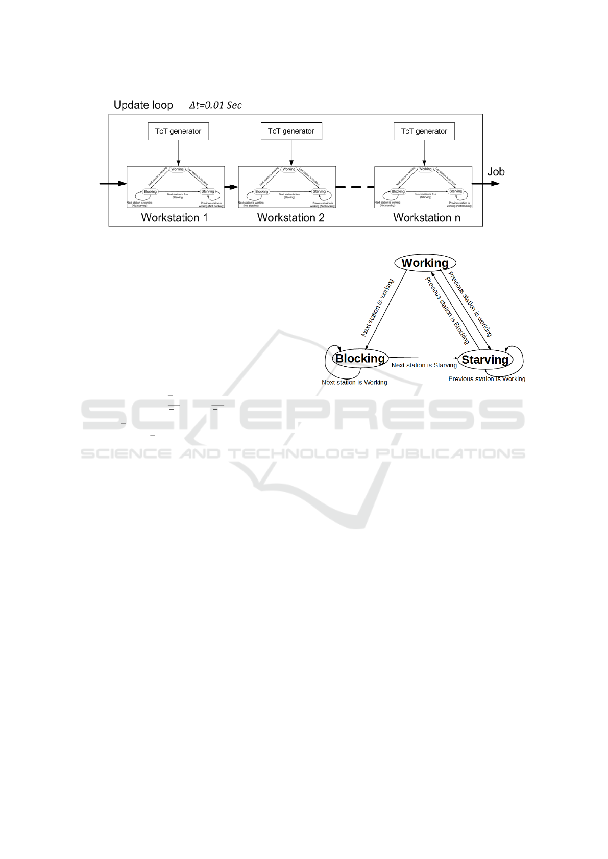
Figure 13: Welding line simulation.

6.1 Welding Line Modelling

The welding line was modeled taking into account the

mini-terms subdivision. that is, the motion of the ro-

bot arm (the time that the robot is in movement), and

the number of welding point for all the 68 different

models and variants, see (E.Garcia, 2016), Anex 4. In

order to adapt the time of each robot is in movement

with the experimental results, thus are recomputed in

cycle time per second, by means of the next equati-

ons;

(8)

Where x

is the mean value without pathology

(Control test) and x

is the mean value for the x pat-

hology. Also in (E.Garcia, 2016), Anex 4, there is

the offset, time that a particular robot is awaiting for

another robot in the same workstation and the trans-

fer time, the required time to move the car body to the

next workstation, (12 seconds). With this model and

using a computer simulation explained below, the pro-

ductivity rate was re-computed in, (E.Garcia, 2016),

taking into account the variability and the production

schedule.

6.2 Welding Line Simulation

The common way to simulate a production line is to

use a simpliﬁed machine state, see Figure 14, with

three possible states, Working, Starving and Blocking.

First of all, let us to deﬁne a serial production line

with three stations, a,b and c, that are chained in this

order. If station b is in Working state and the work is

ﬁnished, it checks station c, if it is in Starving state,

the ﬁnished part of product is delivered to it and sta-

tion b is free to receive another job. If station c is in

Working state when station b ﬁnishes its work, station

b changes its state to Blocking, blocking itself until

station c is free. If station b is free to receive another

part, it checks the previous station. If station a is in

Figure 14: Simpliﬁed state machine.

Working state, station b changes to Starving state wai-

ting until station a has a part to work on. If station a

is in Blocking state, station b receives the part so, the

state of station b changes to Working and the state of

station a changes to Starving. When simulation starts,

every station state is set to Starving, until the ﬁrst sta-

tion is set to Working state. The simulation loop runs

at predeﬁned step time (t). For each step time, the cy-

cle time of each workstation decreases until the cycle

time is zero, meaning that the work is ﬁnished and the

events are triggered.

In order to simulate the welding line, a chain state

machine simulator is developed, see Figure 13. The

loop is updated with an incremental time of 0.01 se-

conds. When the cycle time is ﬁnished in a particu-

lar workstation, a new cycle time is computed for the

next part, taking into account the car model that will

be manufacture in the next cycle. It is important to

point out that there are different mini-terms and repe-

titions of each one for each particular car model deve-

loped in a welding line, see ﬁgure 16.

In the simulated welding line, a job is always per-

formed in the ﬁrst workstation, so that the blocking

state cannot be reached in the ﬁrst station. In addition,

all the ﬁnished jobs in the last workstation are retired,

so that the Starving state cannot be reached in the last

workstation. The loop starts with all the stations in

the Blocking state.

ICINCO 2018 - 15th International Conference on Informatics in Control, Automation and Robotics

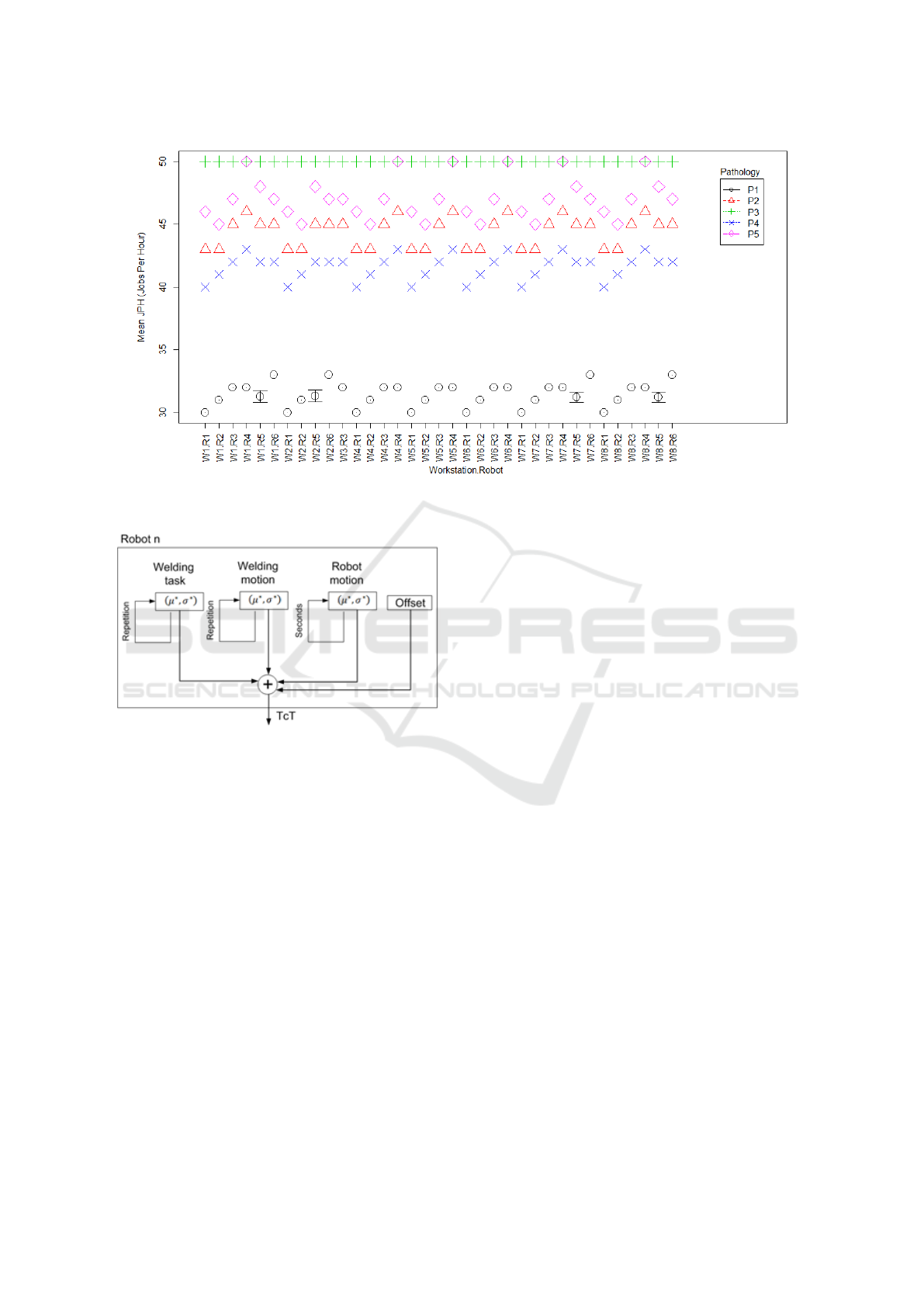
Figure 15: JPH VS Pathologies VS Welding station.

Figure 16: Cycle time computation for each welding unit.

The cycle time for each workstation is the max-

imum cycle time of each welding station that works

in parallel, indicating the slower welding unit and the

bottleneck in a particular workstation.

6.3 Simulation Results

Figure 15 shows the simulation results. As can we

expect, there are a variability between pathologies.

While Pathology 3 has a neglictible effect, nearly to

the ERR of the line, pathology 1 has a deep effect,

reducing the production rate around 32 JPH. Also the

simulation results shows the variability if the patho-

logy apperas in a different welding station, around 4

JPH. This behaviour is due to the dynamic behaviour

of the bottleneck.

The information provided by the simulation could

be useful to prioritize the maintenance tasks after

change point, with the goal to minimize the loss of

productivity.

7 CONCLUSIONS AND FUTURE

WORKS

This paper shows how to design a Knowledge-driven

Maintenance Support System (MSS) to prognosticate

breakdowns in production lines. The system is based

on the sub-cycle time (mini-terms) monitorization and

statistical analysis of the data obtained in the experi-

ments allowing us to deﬁne the rules that govern the

decisions for the real-time Knowledge-driven MSS.

By means of the same statistical analisys and a nu-

merical simulation techniques, it is possible to know

the loss of production rate produced after the change

point. Not only does it allow to predict breakdowns

but it also allows to know the loos of productivity pro-

duced by each pathology.

Our immediate future work is to connect the

Knowledge-driven MSS to the real welding line.

Starting from the initial conﬁguration deﬁned here,

Knowledge-driven MSS could be continuously enri-

ched, tuning the thresholds values and adding new

pathologies and rules to the system. Real-time nume-

rical simulation will allow us to prioritize the mainte-

nance tasks with the goal to minimize the impact in

the production rate.

Moreover, the remaining useful life estimation

(RUL) for each component after change point is anot-

her fact that the Knowledge-driven MSS could learn,

giving an accurate breakdown prognostic and allo-

wing the maintenance team to schedule maintenance

tasks by another priority criteria.

Towards a Knowledge-driven Maintenance Support System for Manufacturing Lines

ACKNOWLEDGEMENTS

The authors wish to thank Ford Espa

na S.L and in

particular Almussafes Factory for the support in the

present research.

REFERENCES

A.Chakir (2016). A decision approach to select the best

framework to treat an it problem by using multi-agent

system and expert systems. Advances in Ubiquitous

Networking, pages 499–511.

A.K.S.Jardine, D. and D.Banjevic (2006). A review on

machinery diagnostics and prognostics implementing

condition-based maintenance. . Mechanical Systems

and Signals processing, 20(7):1483–1510.

E.Garcia (2016). Anlisis de los sub-tiempos de ciclo tcnico

para la mejora del rendimiento de las lneas de fabrica-

cin. PhD.

E.Garcia and N.Montes (2017). A tensor model for automa-

ted production lines based on probabilistic sub-cycle

times. Nova Science Publishers, 18(1):221–234.

H.R.Nemati (2002). Knowledge warehouse: an architec-

tural integration of knowledge management, decision

support, artiﬁcial intelligence and data warehousing.

Decision Support Systems, 33(2):143–161.

K.L.Son (2013). Remaining useful life estimation based on

stochastic deterioration models: A comparative study.

Reliability Engineering and System Safety, 112:165–

175.

L.Li, Q. and J.Ni. (2009). Real time production im-

provement through bottleneck control. International

Journal of production research, 47(21):6145–6158.

M.Chergui (2016). A decision approach to select the best

framework to treat an it problem by using multi-agent

systems and expert systems. Advances in Ubiquitous

Networking, pages 499–511.

M.Murthadha (2013). Knowledge-driven decision support

system based on knowledge warehouse and data mi-

ning for market management. Journal of Management

and Business Research, 13(10):2249–4588.

M.Negnevitsky (2005). Artiﬁcial intelligence: a guide to

intelligent systems. pearson Education.

R.R.Deshpande (2016). Knowledge-driven decision sup-

port for assessing dose distributions in radiation ther-

apy of head and neck cancer. International Jour-

nal of Computational assistant in Radiology Surgery,

11(11):2071–2083.

S.H.Muhammad (2017). Decision support system classiﬁ-

cation and its application in manufactoring sector: A

review. Jurnal Teknologi, 79(1):153–163.

X.Zhao (2014). Localized structural damage detection: A

change point analysis. Computer-Aided Civil and In-

frastructure Engineering, 29:416–432.

X.Zhao (2018). Optimal replacement policies for a shock

model with a change point. Computers & Industrial

Engineering, 118:383–393.

ICINCO 2018 - 15th International Conference on Informatics in Control, Automation and Robotics