Finding Regressions in Projects under Version Control Systems

Jaroslav Bend

ık, Nikola Bene

s and Ivana

Cern

Faculty of Informatics, Masaryk University, Brno, Czech Republic

Keywords:

Version Control Systems, Regressions, Regression Points, Code Debugging, Bisection.

Abstract:

Version Control Systems (VCS) are frequently used to support development of large-scale software projects.

A typical VCS repository can contain various intertwined branches consisting of a large number of commits.

If some kind of unwanted behaviour (e.g. a bug in the code) is found in the project, it is desirable to ﬁnd the

commit that introduced it. Such commit is called a regression point. There are two main issues regarding the

regression points. First, detecting whether the project after a certain commit is correct can be very expensive

and it is thus desirable to minimise the number of such queries. Second, there can be several regression points

preceding the actual commit and in order to ﬁx the actual commit it is usually desirable to ﬁnd the latest

regression point. Contemporary VCS contain methods for regression identiﬁcation, see e.g. the git bisect

tool. In this paper, we present a new regression identiﬁcation algorithm that outperforms the current tools by

decreasing the number of validity queries. At the same time, our algorithm tends to ﬁnd the latest regression

points which is a feature that is missing in the state-of-the-art algorithms. The paper provides an experimental

evaluation on a real data set.

1 INTRODUCTION

Version Control Systems (VCS) have become ubiqui-

tous in the area of (not only) software development,

from small toy projects to large-scale industrial ones.

The recent years saw a rise in the popularity of Dis-

tributed VCS such as git (Git, 2018), bazaar (Bazaar,

2018), Mercurial (Mercurial, 2018) and many others.

These allow for almost seamless cooperation of a large

number of developers and support extensive project

branching and merging of branches. After a project

has been in the development process for some time,

the commit graph of its repository may grow to be very

large.

As projects grow larger, the appearance of bugs

(i.e. unwanted behaviour of the developed product) is

going to be inevitable. Software bugs can be usually

caught early if the development teams employ exten-

sive testing techniques (unit tests, performance regres-

sion tests, etc.); however, from time to time a bug, or

a commit that changed properties of the project, may

creep into the VCS repository and lie there undetected

for some time. Such bug is usually discovered by

e.g. extending the coverage of the tests or by employ-

ing some other veriﬁcation technique such as model

checking (Clarke et al., 2001). In order to ﬁx the bug

it is very useful to identify the commit that introduced

the bug as this commit typically contains a relatively

small set of source code changes. It is much easier to

properly understand and ﬁx a bug when you only need

to check a very small set of changes of the source code.

Sometimes we are not looking for the commit that

introduced a bug, but rather for a commit that caused

a change between some “old” and “new” state of the

project. As an example, we might be looking for the

commit that introduced a particular ﬁx. In such cases

it can seem confusing to use the terms “correct” and

“buggy” to refer to the state before and after the change,

respectively. We thus instead use the terms valid and

invalid commit; we further use the term regression

point to denote the point where the property of interest

has been changed.

The problem of ﬁnding regression points has been

addressed before and there have been developed tools

for solving this problem, such as git bisect (Git bi-

sect documentation, 2018). These tools have proved

themselves to be very useful and are commonly used

during software development nowadays. Yet, there are

several issues related to ﬁnding regression points and

only some of them are targeted by the state-of-the-art

tools.

First, the search for regression points consists of

several queries of the form: “Given a certain commit,

is the bug present in the system after this commit?”

Such queries, which we call validity queries, may con-

sist of several expensive tasks like running tests, model

152

Bendík, J., Beneš, N. and

Cerná, I.

Finding Regressions in Projects under Version Control Systems.

DOI: 10.5220/0006864401520163

In Proceedings of the 13th International Conference on Software Technologies (ICSOFT 2018), pages 152-163

ISBN: 978-989-758-320-9

checking, code inspection, or other forms of veriﬁca-

tion. It is thus desirable to minimise the number of

these queries. Second, the validity of commits does

not, in general, have to be monotone. Perhaps a bug

was introduced in a certain commit, inadvertently ﬁxed

several commits later, and then reintroduced in a yet

later commit. This means that there are possibly sev-

eral regression points preceding the actual invalid com-

mit, but only the identiﬁcation of the latest regression

point can usually help us to ﬁx the bug. The third issue

concerns large projects with many branches. If, for

example, a new test case is employed, then more than

just one active branch can fail the test case and it is de-

sirable to identify a regression point for each of these

branches. We can ﬁnd the regression point for each

branch separately. However, dealing with all branches

simultaneously can save some validity queries and thus

optimise the search.

The state-of-the-art tools target the need to min-

imise the number of validity queries that are performed.

However, they do not tend towards identiﬁcation of lat-

est regression points, and they deal with only a single

invalid branch at a time.

The goal of this paper is to provide a novel algo-

rithm, called the Regression Predecessors Algorithm

(RPA), that solves the problem of ﬁnding regression

points in VCS repositories. The algorithm minimises

the number of validity queries and at the same time

tries to ﬁnd the latest regression points both for single

and multiple invalid branches. RPA has several vari-

ants which we compare on a set of real open-source

projects. Moreover, we compare the RPA algorithm

with the state-of-the-art tool git bisect and demonstrate

that our algorithm outperforms git bisect in all of the

three above-mentioned criteria: in the number of per-

formed validity queries, in ﬁnding the latest regression

points, and in ﬁnding regression points for multiple

invalid branches.

1.1 Example Use Case

Let us describe a common situation from the area of

web development in which RPA can be used. Assume

a small company that develops a content management

system (CMS) for eCommerce. Such a CMS typi-

cally consists of several features, e.g. product man-

agement, discount system, or customer management.

Many of these features are furthermore divided into

sub-features; for example the discount feature can be

divided into buy one, get one free discounts, coupon

based free shipping discounts, order-speciﬁc discounts,

and seasonal discount. At the beginning, only basic

features are available and the remaining features are

gradually developed. The company uses a version con-

trol system, e.g. git, and uses branching to separate

development of individual features.

Some parts of the CMS are based on JavaScript,

e.g. an interactive shopping cart page. The usage

of JavaScript provides several advantages, but it also

brings some disadvantages. One of the major disad-

vantages is that different web browsers may interpret

JavaScript code differently which may result in unac-

ceptable inconsistencies in terms of functionality and

interface. At the end of the day, the company has to

ensure that all recent versions of all the major web

browsers provide the same functionality.

The problem is that JavaScript envolves, i.e. new

versions are released, and it usually takes months till

all the major web browsers support a particular ver-

sion of JavaScript. Some features of JavaScript even

never get supported by some browsers. Assume that

a developer used a JavaScript directive in a moment

when some browsers support the directive and the oth-

ers ignore it, i.e. it helps in some browsers and it

does no damage in the others. Several months later,

a browser from the latter group starts to support the

directive, however it interprets it in a different way

than the other browsers, which causes a bug. It is very

likely that the developer used the directive repeatedly

in different pieces of code and that these pieces were

subsequently adopted by some of the features that are

currently being developed, i.e. the bug is presented in

several active branches. It is also easy to imagine that

this particular bug was introduced in a certain commit,

ﬁxed several commits later during code refactoring,

and then maybe reintroduced in a yet another commit.

The rest of the paper is organised as follows. Sec-

tion 2 deﬁnes basic notions and states the problem

formally. Section 3 presents the Regression Predeces-

sors Algorithm and illustrates its behaviour on a small

example. Section 3.5 reviews the related work and

compares RPA with other known algorithms. Section 4

gives an experimental evaluation of different variants

of RPA and compares RPA with the state-of-the-art

tool git bisect on a set of real benchmarks.

2 PRELIMINARIES AND

PROBLEM FORMULATION

Deﬁnition 1.

A rooted directed acyclic graph is

a directed graph

G = (V, E)

with exactly one root

(i.e. a vertex with no incoming edges) and with no

cycle (i.e. there is no path

, v

, ···v

in the graph

such that

= v

and

k > 0

). A rooted annotated di-

rected acyclic graph (RADAG) is a pair

(G, valid)

where

is a rooted directed acyclic graph with root

Finding Regressions in Projects under Version Control Systems

153

Figure 1: An example of a RADAG, the dashed vertices

are invalid. There are three invalid leaves in this example:

, and four regression points:

(c, d), (e, h),(n, i)

and

(o, p)

. The ﬁrst three regression points are regression prede-

cessors of invalid leaves

k, m

; the fourth regression point is

the regression predecessor of the invalid leaf p.

and

valid : V → Bool

is a validation function satisfying

valid(r) = True.

We use RADAGs to model structures which arise

from using version control systems (VCS). Each vertex

corresponds to a commit in VCS repository. An

edge between two vertices represents two subsequent

commits. The root corresponds to the initial commit

and the leaves (vertices with no outgoing edges) corre-

spond to the latest commits of individual branches.

The validation function expresses whether a partic-

ular commit has the desired property that the system

after this commit is correct (i.e. does not contain the

bug). We call the vertices with this property (for which

the validation function evaluates to

True

) valid vertices

and the others invalid ones. Note that we assume that

the graph has only one root and that the root is valid.

If this is not the case, the graph can be easily modiﬁed

by adding a dummy initial valid commit.

Deﬁnition 2.

A regression point of a RADAG

((V, E),valid)

is a pair of vertices

(u, v)

such that

(u, v) ∈ E

valid(u) = True

, and

valid(v) = False

. A re-

gression point

(u, v)

is a regression predecessor of

a vertex

w ∈ V

is equal to

is reachable from

We are now ready to formally state our problem.

Regression Predecessors Problem:

Given

a RADAG

(G, valid)

and a set of invalid leaves

ﬁnd at least one regression predecessor for each leaf

from L.

Note that one invalid leaf can have several regres-

sion predecessors and one regression point can be a re-

gression predecessor of several invalid leaves. There-

fore, the regression predecessors problem may have

several different solutions. For an example of such

a RADAG see Figure 1.

3 REGRESSION PREDECESSORS

ALGORITHM (RPA)

A naive solution to the regression predecessors prob-

lem would be to evaluate the function

valid

for each

vertex, identify all regression points in

, and ﬁnd a

regression predecessor of each invalid leaf using the

reachability relation. Because this approach identiﬁes

all regression points we can choose the latest regres-

sion predecessor of every invalid leaf. However, the

price is crucial; the function

valid

is evaluated for

every vertex which is assumed to be extremely time-

consuming.

In this section we present a new algorithm, the

Regression Predecessors Algorithm (RPA), that sub-

stantially decreases the number of vertices for which

the function

valid

is evaluated and tends to ﬁnd the

latest regression points at the same time.

3.1 Basic Schema

The main idea of RPA is based on the observation

that if a leaf

is invalid then every path starting in

a valid vertex and leading to

must contain at least one

regression predecessor of

. This reduces the problem

to two tasks: ﬁnding a path and detecting a regression

point on the path.

For the basic description of RPA see Algorithm 1.

The algorithm maintains the set

UnprocessedLeaves

which consists of those invalid leaves for which a re-

gression predecessor has not been computed yet. The

set

KnownValid

consists of those vertices for which

the function

valid

has been evaluated and are valid

(initially only the root is known to be valid). In each

iteration, the algorithm chooses a leaf

from the set

UnprocessedLeaves

. A regression predecessor of

acquired by building a path

which connects a valid

vertex x ∈ KnownValid with l and by ﬁnding a regres-

sion point

(u, v)

on this path. While searching for

the regression point

(u, v)

, the function

valid

is eval-

uated for some vertices on the path

. The newly

detected valid vertices form a set

NewValid

and the set

KnownValid is updated accordingly.

The algorithm also exploits the fact that one regres-

sion point can be a regression predecessor of several

invalid leaves. Therefore, every time a regression point

(u, v)

is found, it is propagated to every invalid leaf

m ∈ UnprocessedLeaves

such that

reachable from

. Every such

is removed from

UnprocessedLeaves

After this propagation step, the procedure also removes

from the graph all vertices reachable from

. By re-

moving vertices we avoid propagation of regression

points to leaves for which a regression predecessor has

already been found and avoid unnecessary traversal of

ICSOFT 2018 - 13th International Conference on Software Technologies

154

1 function RPA(G, L)

input: a RADAG G = ((V, E), valid : V → Bool) with root r

input: a set of invalid leaves L

output: a regression predecessor for each leaf l ∈ L

2 UnprocessedLeaves ← L

3 KnownValid ← {r}

4 while UnprocessedLeaves 6=

0 do

5 l ← a leaf from UnprocessedLeaves

6 UnprocessedLeaves ← UnprocessedLeaves \ {l}

7 p

← a path hx, . . . , li such that x ∈ KnownValid

8 (u, v) ← ﬁnd a regression point on p

9 KnownValid ← KnownValid ∪ NewValid

10 output (u, v) is a regression predecessor of l

11 propagateRegressionPoint(v, (u, v)) // optional, Alg. 2

Algorithm 1: Regression predecessors algorithm (basic schema).

1 function propagateRegressionPoint(k, (u,v))

input: a regression point (u, v)

input: a vertex k reachable from v (or v = k)

2 for (k, l) ∈ E do

3 propagateRegressionPoint(l, (u,v))

4 if k ∈ UnprocessedLeaves then

5 output (u, v) is a regression predecessor of k

6 UnprocessedLeaves ← UnprocessedLeaves \ {k}

7 remove k from the graph

Algorithm 2: Regression point propagation.

the graph. For a complete description of the procedure,

see Algorithm 2.

On the one hand, the propagation can result in sav-

ing some validation calls. On the other hand, the use

of propagation may be in conﬂict with the desire to

identify the latest regression predecessors. Therefore,

the usage of propagation is optional. Section 4 demon-

strates the behaviour of the algorithm both with and

without the propagation step.

There are further three key aspects that affect the ef-

ﬁciency of the algorithm: the order in which leaves are

chosen from the set

UnprocessedLeaves

, the method

of building the path connecting a valid vertex with

the invalid leaf, and the method of regression points

identiﬁcation. We focus on these three aspects in the

following text.

3.2 Identiﬁcation of Regression Points

In this subsection we give the details of our solution

to the problem of ﬁnding a regression point on a given

path

p = hv

, v

, . . . , v

connecting a valid vertex

with an invalid vertex v

Linear Search.

The simplest solution to the task is

to evaluate the function

valid

for each vertex on the

path, starting with

and going backwards. As soon

as a valid vertex

is found, the algorithm outputs

, v

i+1

)

as a regression predecessor of

. By start-

ing with

and going backwards we guarantee that

, v

i+1

)

is the nearest regression point of

along this

path. The disadvantage of this approach is that in the

worst case all vertices on the path are tested for validity.

Because the commit graphs of VCS usually contain

hundreds or thousands of commits and the evaluation

of the function valid is assumed to be very expensive,

the linear search is practically unusable.

Binary Search.

Provided that the ﬁrst vertex of the

path is valid and the last is invalid (which is always

our case) we can use binary search to ﬁnd a regression

point. Let

p = hv

, v

, . . . v

mid

, . . . , v

be a path such

that

is valid,

is invalid, and

mid

is the middle

vertex of this path. If

mid

is valid then there is a re-

gression point on the path

mid

, . . . , v

. Otherwise,

there is a regression point on the path

, . . . v

mid

. We

can thus always reduce

into half and recursively re-

Finding Regressions in Projects under Version Control Systems

155

1 function multSearch(p)

input: a path p = hv

, . . . , v

i with valid v

and invalid v

output: a regression point contained in p

2 if l = 1 then

3 return (v

, v

)

4 k = 1

5 while l − (2

− 1) > 0 do

6 if valid(v

l−(2

−1)

) then

7 return multSearch(hv

l−(2

−1)

, . . . , v

l−(2

k−1

−1)

8 k = k + 1

9 return multSearch(hv

, . . . , l − (2

k−1

− 1)i)

Algorithm 3: Multiplying search.

peat the procedure. Eventually, we end up with a path

of length 2, thus a regression point is found.

Contrary to the linear search it is not guaranteed

that the binary search ﬁnds the regression point which

is nearest to

. The main advantage of the binary

search is that it always performs logarithmically many

checks, since the path is in each iteration reduced

by half. Its efﬁciency is not much affected by the

position of the regression points on the path.

Multiplying Search.

The so-called multiplying

search approach combines the advantages of both

binary and linear search approaches as it performs

asymptotically fewer validity checks than the linear

search and at the same time tends to ﬁnd a regres-

sion point which is closer to the last vertex

than the

regression point found by the binary search.

Let

p = hv

, v

, . . . , v

be a path such that

valid and

is invalid. The multiplying search ﬁrst

evaluates the function

valid

for the vertex

l−1

. If

l−1

is not valid, then the function is stepwise evaluated

for vertices

l−(2

−1)

l−(2

−1)

l−(2

−1)

, . . .

forming

exponentially large gaps between individual vertices.

The procedure eventually ﬁnds an

such that the ver-

tex

l−(2

i−1

−1)

is invalid and either

l−(2

−1)

is valid

l − (2

− 1) < 0

. If the former happens, then the

procedure recursively continues with the new path

p = hv

l−(2

−1)

, v

l−(2

−2)

, . . . , v

l−(2

i−1

−1)

. In the latter

case the procedure recursively continues with the path

p = hv

, v

, . . . , v

l−(2

i−1

−1)

. The procedure converges

to a path containing only two vertices such that the

ﬁrst vertex of the path is valid and the second invalid,

i.e., a regression point is found. For the complete

description see Algorithm 3.

The number

C(n)

of vertices on which the function

valid

is evaluated on a path of length

is bounded by

the recurrence equation

C(n) ≤ C(

) + log n

. In each

recursive call the number of evaluations is at most

logn

and the length of the path is decreased at least by

half. The solution of the recurrence equation (using

the Master theorem (Verma, 1994)) gives an upper

bound

O(log

on the number of vertices on which

the function valid is evaluated.

Note that multiplying search can signiﬁcantly out-

perform binary search in many cases. Its perfor-

mance depends on the distance of the regression points

from the leaf. The closer are the regression points to

the leaf, the more likely multiplying search outper-

forms binary search. For example, assume two paths

= hv

, v

, . . . , v

1023

= hv

, v

, . . . , v

1023

, where

1007

, v

1008

)

is the only regression point of

and

512

, v

513

)

is the only regression point of

. The bi-

nary search approach performs

validity queries on

both paths whereas the multiplying search approach

performs 6 queries on p

and 17 queries on p

3.3 Leaf Selection and Path

Construction

Our next goal is to specify the order in which unpro-

cessed leaves are chosen and determine the method

of building a path connecting a valid vertex with the

chosen leaf.

We assume that the directed acyclic graphs induced

by VCS are represented using adjacency lists (see (Cor-

men et al., 2009)) in which every vertex is equipped

both with a list of its direct successors and a list of its

direct predecessors. In the initialisation phase of RPA

we compute the length of the shortest paths from

for each vertex

v ∈ V

and invalid leaf

l ∈ L

. For every

pair

(v, l) ∈ V × L

we maintain a successor of

so that

the chain of successors originating at the vertex

runs

forward along a shortest path from

. This com-

putation is done by running a backwards breadth-ﬁrst

search from each

l ∈ L

using the list of predecessors,

for details see e.g. (Cormen et al., 2009).

ICSOFT 2018 - 13th International Conference on Software Technologies

156

1 function priorityBasedRPA(G, L)

input: a RADAG G = ((V, E), valid : V → Bool) with root r

input: a set of invalid leaves L

output: a regression predecessor for each leaf l ∈ L

2 for each (v, l) ∈ V × L compute the value dist(v, l)

3 for each l ∈ L do

4 dist(l) ← dist(r, l)

5 start(l) ← r

6 UnprocessedLeaves ← L // priority queue

7 while UnprocessedLeaves 6=

0 do

8 l ← UnprocessedLeaves.dequeueMinimum()

9 p

← a shortest path hx, . .. , li such that x = start(l)

10 (u, v) ← ﬁnd a regression point on p

11 KnownValid ← KnownValid ∪ NewValid

12 output (u, v) is the regression predecessor of l

13 propagateRegressionPoint(v, (u, v)) // optional, Alg.2

14 updatePriorities(NewValid) // Alg.5

Algorithm 4: Regression predecessor algorithm.

In what follows we use

dist(v, l)

to denote the

length of the shortest path leading from the vertex

v to the leaf l; we further deﬁne:

dist(l) = min{dist(u, l) | u ∈ KnownValid}

start(l) = u such that u ∈ KnownValid

and dist(u, l) = dist(l).

In other words,

dist(l)

denotes the length of a shortest

path leading to

from a vertex

for which the function

valid

has been evaluated and is valid (i.e. belongs to

the set

KnownValid

). The ﬁrst vertex of such a path

is denoted

start(l)

. As the set

KnownValid

changes

during the computation, so may the values

dist(l)

and

start(l)

. Initially, only the root

of the graph is known

to be valid, therefore

dist(l) = dist(r, l)

and

start(l) =

r for each l ∈ L.

The way in which RPA ﬁxes the order in which in-

valid leaves are processed and determines which paths

should be used for identiﬁcation of regression points is

based on the following observation. The shorter path

we process the fewer number of evaluations of the

function

valid

is performed, independent on the regres-

sion ﬁnding approach. For a complete description of

the RPA algorithm see Algorithm 4, for an illustrative

example see Section 3.4.

The RPA algorithm maintains the set

UnprocessedLeaves

as a priority queue where

each

l ∈ UnprocessedLeaves

is assigned the priority

dist(l)

. In every iteration the algorithm extracts the

leaf

with minimum priority from

UnprocessedLeaves

and constructs the shortest path leading to

. More-

over, each iteration is supplemented by the method

updatePriorities(newValid)

that updates the

dist(l)

and start(l) values (see Algorithm 5).

1 function updatePriorities(NewValid)

input: A set of valid vertices NewValid

2 for each v in NewValid do

3 for each lea f ∈ UnprocessedLeaves

4 if dist(v, lea f ) < dist(lea f ) then

5 start(lea f ) ← v

6 dist(lea f ) ← dist(v, lea f )

Algorithm 5: Priority update.

3.4 Example

Figure 2 demonstrates the execution of RPA with mul-

tiplying search and propagation. In this example, the

RADAG has only invalid leaves,

L = {g, k, m, p}

, and

the task is to ﬁnd the regression predecessors for all

leaves. The computation consists of 3 iterations. The

function

valid

is evaluated only for 7 out of 16 vertices

and 3 regression points are found. We list the values of

control variables in each iteration and illustrate them

on the graph. The vertices on which the

valid

function

has been evaluated are ﬁlled with green or red color de-

pending on their validity. The vertices removed from

the graph are shaded.

3.5 Related Work

To the best of our knowledge, the ﬁrst tool for ﬁnd-

ing regression points was the git bisect tool (Git bi-

sect documentation, 2018) which is a part of the dis-

tributed VCS git (Git, 2018). The method used in

the git bisect tool is called bisection and it was sub-

Finding Regressions in Projects under Version Control Systems

157

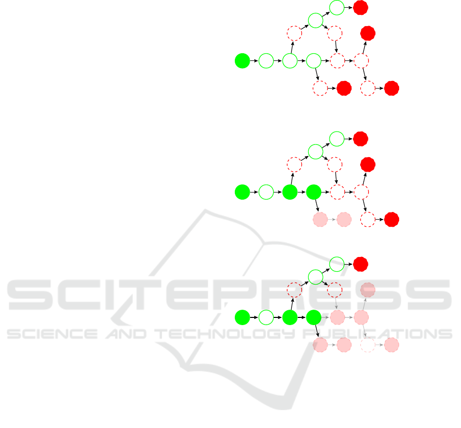
I. iteration

– Removed vertices =

– KnownValid = {a}

– Priority queue = hp, g, k, mi

– dist(p) = 5, dist(g) = 6,

dist(k) = 6, dist(m) = 7

– start(p) = a

– path p

= ha, b, c, n, o, pi

– Tested vertices: o, c, n

– Regression point of p

= (n, o)

– Propagated to: {p}

II. iteration

– Removed vertices = {o, p}

– KnownValid = {a, c, n}

– Priority queue = hk, m, gi

– dist(k) = 3, dist(m) = 4, dist(g) = 4

– start(k) = n

– path p

= hn, i, j, ki

– Tested vertices: j, i

– Regression point of p

= (n, i)

– Propagated to: {k, m}

III. iteration

– Removed vertices = {o, p, i, j, k, l, m}

– KnownValid = {a, c, n}

– Priority queue = hgi

– dist(g) = 4

– start(g) = c

– path p

= hc, d, e, f , gi

– Tested vertices: f

– Regression point of p

= ( f , g)

– Propagated to: {g}

Figure 2: An illustrative example.

sequently adopted by other VCS like Mercurial (Mer-

curial, 2018), Subversion (Pilato et al., 2008), and

Bazaar (Bazaar, 2018).

The bisection algorithm takes as an input a sin-

gle invalid commit and ﬁnds a regression point that

precedes this commit. We provide only a brief de-

scription of the bisection algorithm here, for a more

elaborated description please refer to (Git bisect algo-

rithm overview, 2018). The algorithm represents the

commits using a directed acyclic graph and assumes

that the function

valid

is monotone, i.e. that every suc-

cessor of an invalid commit is also invalid. It starts by

taking as an input a single invalid commit called “bad”

together with a one or more commits which are known

to be valid. Then, it iteratively repeats the following

steps:

(i)

Keep only the commits that: a) precede “bad” com-

mit (including the “bad” commit itself) and b) do

not precede a commit which is known to be valid

(excluding the commits which are known to be

valid).

(ii)

Associate to each commit

a number

r = min{(x +

1), n − (x + 1)}

where

is the number of commits

that precede the commit

and

is the total number

of commits in the graph. Roughly speaking, this

number represents the amount of information that

can be obtained by evaluating the function

valid

. If

is valid then all of its predecessors are

necessarily also valid (based on the assumption

that the function

valid

is monotone). In the other

case, if

is invalid, then all of its successors are

necessarily also invalid.

(iii)

Evaluate the function

valid

for the commit

with

the highest associated number. If

is invalid then

it becomes the “bad” commit.

Eventually there will be only one invalid commit

left in the graph with one of its predecessors in the

ICSOFT 2018 - 13th International Conference on Software Technologies

158

original graph being valid. This pair of vertices forms

the regression predecessor of the original “bad” com-

mit. Although the main idea of the bisection method is

based on the monotonicity of the function

valid

, it is

guaranteed that the algorithm ﬁnds a regression prede-

cessor of the “bad” commit even if the function

valid

is not monotone.

There are two main drawbacks of git bisect com-

paring to RPA. First, the bisection algorithm does not

tend to ﬁnd the latest regression predecessor. Second,

experiments (see the following section) demonstrate

that git bisect evaluates more commits than RPA. The

reason of this behaviour is that RPA prefers shortest

paths while git bisect prefers vertices with the high-

est associated number. To demonstrate the difference

let us consider a graph with one leaf and two paths

connecting the root with the leaf. If one path is very

short and the second one very long, then RPA prefers

the short path while git bisect evaluates vertices on the

long one. If a graph contains only one path leading to

an invalid leaf, git bisect evaluates the same vertices

as RPA combined with binary search.

There is also further related work that deals with

problems similar to ours. Heuristics for automated

culprit ﬁnding (Ziftci and Ramavajjala, 2015) are used

for isolating one or more code changes which are

suspected of causing a code failure in a sequence of

project versions. They assume that the codebase is

tested/validated regularly (e.g. after every n commits)

using some test suit. If a bug is detected, they search

for the culprit only among the changes to the codebase

that have been made since the latest appliance of the

test suite. The individual versions are rated accord-

ing to their potential to cause the failure (e.g. versions

with many code changes are rated higher) and versions

with high rate are tested as ﬁrst. The culprit ﬁnding

technique (Ziftci and Ramavajjala, 2015) is efﬁciently

applicable only for searching in a short term history

and it assumes that there is only one culprit.

Delta debugging (Zeller, 1999) is a methodology

to automate the debugging of programs using the ap-

proach of a hypothesis-trial-result loop. For a given

code and a test case that detects a bug in the code, the

delta debugging algorithm can be used to trim useless

functions and lines of the code that are not needed

to reproduce to bug. The delta debugging cannot be

used for ﬁnding regression points in VCS. However,

we believe that it can be incorporated into RPA and

improve its performance by reducing the portion of

code that need to be validated by the function valid.

A regression testing (Agrawal et al., 1993) and con-

tinuous integration testing (Duvall, 2007) are types of

software testing that veriﬁes that software previously

developed and tested still performs correctly even af-

ter it was changed or interfaced with other software.

These two techniques are suitable for ﬁxing bugs that

are detected right after they are introduced. However,

if a bug that lied in a codebase for some time is de-

tected, e.g. because of extending the coverage of the

tests, a technique like RPA need to be used. That

is, RPA and regression testing/continous integration

testing are mutually orthogonal techniques

SZZ (Sliwerski et al., 2005; Kim et al., 2006) is

an algorithm for identifying commits in a VCS that

introduced bugs, however it works in a quite different

settings. It assumes, that the bug has been already ﬁxed

and that the commit that ﬁxed the bug is explicitly

known or can be found in a log ﬁle. This allows to

identify particular lines of code that ﬁxed the bug and

this information is then exploited while searching for

the bug-introducing commit. In our settings, the bugs

are not ﬁxed yet, thus SZZ cannot be used.

In our previous work (Bend

ık et al., 2016), a struc-

ture similar to RADAG appears. However, that struc-

ture is monotone and therefore, the problem formu-

lated in (Bend

ık et al., 2016) substantially differs from

the regression predecessors problem and the algorithm

presented in that work cannot be used for ﬁnding re-

gression points in RADAGs.

Finally, we relate the regression predecessors prob-

lem with well known problems from graph theory. The

latest regression point can be found using the breadth-

ﬁrst-search (BFS) algorithm (Jungnickel, 1999). As

our goal is to minimize the number of validity queries,

BFS is not suitable as it queries every vertex. There-

fore, we come with a new, specialized, algorithm.

4 EXPERIMENTAL RESULTS

We demonstrate the performance of the variants of

RPA on two types of use cases. We ﬁrst focus on the

problem of ﬁnding a regression predecessor of a single

invalid leaf. We then focus on the problem of ﬁnding

regression predecessors of a set of invalid leaves. We

also compare the performance of the RPA variants to

that of the git bisect tool (Git bisect documentation,

2018; Git bisect algorithm overview, 2018).

As benchmarks we use large real open source

projects, taken from the GitHub open source show-

cases (Github Showcases, 2018), with at least 8 ac-

tive branches or at least 1000 commits. Due to the

size of the projects it would be intractable to build

and test all commits in these projects. Therefore we

use those projects from (Github Showcases, 2018)

that employ TravisCI (Travis CI, 2018). Travis CI

is a service used to build and test projects hosted at

GitHub and the results of all tests that were run on

Finding Regressions in Projects under Version Control Systems

159

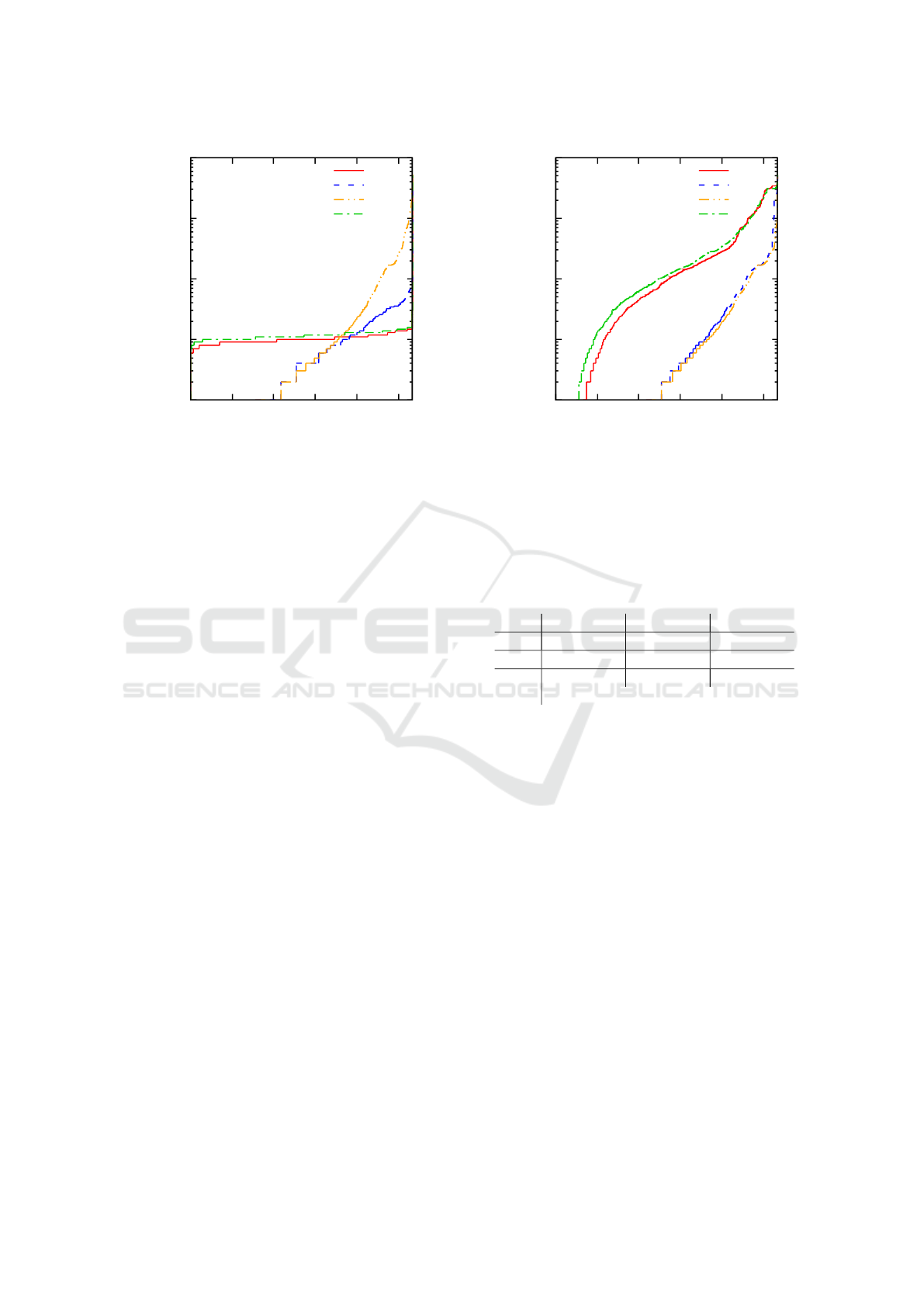
100

1000

10000

0 200 400 600 800 1000

Number of validity queries

Number of instances

RPA binary search

RPA multiplying search

RPA linear search

git bisect

Figure 3: Cumulative distribution plot of performed validity

queries for each evaluated algorithm. A point with coordi-

nates [x,y] can be read as “x instances were solved by using

at most y validity queries”.

these projects are publicly available. Whenever our

algorithm needs to validate a commit, it acquires the

results of the tests from the publicly available Travis

CI database instead. Overall we selected 84 projects

with 1069 invalid leaves in total. Our selection in-

cludes for example the Rails web-application frame-

work (Ruby on Rails, 2018; B

achle and Kirchberg,

2007), the PHP Interpreter (PHP interpreter, 2018), or

the ArangoDB (ArangoDB, 2018).

We do not provide any details about the architec-

ture of the computer on which we run the experiments

because the computation time is not a relevant crite-

rion in our study. It took a few seconds to run all the

experiments because we didn’t actually run the tests.

As a main criterion for measuring the efﬁciency of

evaluated algorithms we use the number of performed

validity queries and the distance between identiﬁed

regression points and corresponding invalid leaves (in

order to measure the tendency to ﬁnd the latest regres-

sion points). Complete results of all measurements are

available at https://tinyurl.com/y7ps4yyl.

4.1 Single Invalid Leaf Instances

We ﬁrst analyse how variants of RPA and git bisect

perform while searching for a regression predecessor

of a single invalid leaf. In the case of ﬁnding a re-

gression predecessor of a single invalid leaf, it makes

no sense to use propagation. Therefore, we always

build the shortest path from a valid vertex and employ

either binary or multiplying search. We also include

the naive linear search approach that builds a path and

checks one by one individual commits on the path.

100

1000

10000

0 200 400 600 800 1000

Distance of a regression point from the leaf

Number of instances

RPA binary search

RPA multiplying search

RPA linear search

git bisect

Figure 4: Cumulative distribution plot of distance between

regression predecessor and corresponding invalid leaf for

each evaluated algorithm. A point with coordinates [x,y] can

be read as “in x instances the distance was at most y”.

Table 1: The number of instances on which the algorithm

named in the row performed strictly less validity queries than

the other algorithms. We use the following abbreviations:

mult = RPA with multiplying search, bin = RPA with binary

search, git = git bisect.

< mult bin git

mult — 736 (69%) 759 (71%)

bin 313 (29%) — 824 (77%)

git 294 (28%) 25 (2%) —

The results comparing the number of the performed

validity queries are shown in Fig. 3. In this plot, we

show the cumulative distributions of the performed

validity queries for each evaluated algorithm. The per-

formance of git bisect and binary search was quite

stable on all instances since they always perform log-

arithmically many validity queries. In particular, git

bisect and binary search needed to perform at most 17

and 16 validity queries, respectively, to solve the hard-

est instances. The performance of multiplying search

was less stable, since the number of performed valid-

ity queries depends on the position of the regression

points as we have discussed in Section 3.2. Multiply-

ing search needed to perform from 1 to 101 validity

queries. Linear search was negligibly better than mul-

tiplying search on instances where the regression point

was quite close, however it needed to perform up to

3458 validity queries on the harder instances.

In addition to the plot of cumulative distribution we

show in Table 1 the number of instances on which one

algorithm performed strictly less validity queries than

its competitors. The table shows that binary search was

superior to git bisect on most of the instances. This

ICSOFT 2018 - 13th International Conference on Software Technologies

160

Table 2: The number of instances on which the algorithm

named in the row found a strictly closer regression predeces-

sor than the other algorithms. We use the following abbrevi-

ations: mult = RPA with multiplying search, bin = RPA with

binary search, git = git bisect.

< mult bin git

mult — 717 (67%) 843 (79%)

bin 26 (2%) — 511 (48%)

git 27 (3%) 328 (30%) —

is caused by the nature of these two algorithms. Both

of them need to perform just logarithmically many

validity queries, but git bisect searches the whole graph

whereas binary search traverses only a single path.

Moreover, RPA always chooses the shortest usable

path which might lead to a signiﬁcant improvement to

git bisect. In particular, in some instances, git bisect

performed 3 times more validity queries than RPA with

binary search. On the other hand, RPA with binary

search needed to perform only 1.14 times more validity

queries than git bisect in the worst case. Multiplying

search was strictly better then its competitors on about

70 percent of instances. It was worse on the instances

with large paths where regression points are relatively

far from the leaves.

Besides the number of performed validity queries,

we also measure the tendency of the algorithms to ﬁnd

the latest regression predecessors. So far we have not

precisely deﬁned which regression predecessor is the

latest one and there is more than one suitable deﬁni-

tion. In the case of binary, multiplying, and linear

search we look for a regression predecessor on a path;

thus, we can say that the latest regression predecessor

is the regression point which is closest to the end of

the path (i.e., closest to the leaf). In our experiments,

multiplying search found the closest regression prede-

cessor on the path in 86 percent of instances whereas

binary search only in 29 percent of instances. This

notion of latest regression predecessor is not applica-

ble to git bisect because git bisect does not operate on

paths. In order to compare RPA with git bisect, we

measured the distance between the found regression

predecessor and the corresponding invalid leaf, i.e. the

shortest path between these two vertices in the commit

graph. Fig. 4 shows a plot of cumulative distributions

of distance between regression predecessors and cor-

responding leaves for each evaluated algorithm. The

results demonstrate that multiplying search substan-

tially outperforms binary search and git bisect, and

that binary search is better than git bisect. The naive

linear search is just negligibly better than multiplying

search.

In addition, Table 2 shows the number of instances

on which one algorithm found strictly closer regression

point than its competitors. The multiplying search

strictly dominates both its competitors; the regression

predecessor found by multiplying search was closer to

the leaf than the one found by git bisect in 79 percent

of instances. Binary search performed slightly better,

it was dominated by multiplying search only in 67

percent of instances.

4.2 Sets of Invalid Leaves

We now demonstrate the performance of the RPA vari-

ants on the problem of ﬁnding regression predecessors

for a set of invalid leaves. In particular, we evaluate

both proposed approaches for ﬁnding regression points,

i.e., the binary and multiplying search. Moreover, we

evaluate both these approaches in two variants: with

and without regression point propagation (the optional

part of RPA).

We also compare the variants of RPA to the git bi-

sect tool. As mentioned in Section 3.5, git bisect deals

with the problem of ﬁnding a regression predecessor

of a single invalid leaf. Therefore, in order to solve the

problem of regression predecessors for a given set of

invalid leaves

, git bisect has to be run once per each

leaf from

. As all these runs are independent, it might

happen that some commits are evaluated repeatedly.

In order to avoid the repeated evaluations, we supple-

ment git bisect with a cache saving the results of the

previous evaluations. Thus, every commit is evaluated

at most once.

As benchmarks we used the 84 projects from

GitHub showcases; the goal was to ﬁnd a regression

predecessor for every invalid leaf in every project. In

this part of experimental evaluation we focus solely on

the number of performed validity queries. Figures 5

and 6 show the cumulative distribution plots of the per-

formed validity queries for the variants of RPA with

and without propagation, respectively. In both plots we

also include the results achieved by git bisect. More-

over, we include the cumulative distribution of the

number of invalid leaves (solid black line), i.e. a point

with coordinates

[x, y]

means that

instances have at

most y invalid leaves.

In general, the regression point propagation signiﬁ-

cantly reduces the overall number of performed valid-

ity queries. Considering the difference in performance

between variants of RPA with multiplying and binary

search, respectively, we observe the same behaviour as

in the case of ﬁnding regression predecessors for sin-

gle invalid leaves. There are some instances on which

multiplying search outperformed binary search, and

some instances on which binary search outperformed

multiplying search. The improvement to git bisect is

for both variant of RPA even more signiﬁcant than in

Finding Regressions in Projects under Version Control Systems

161

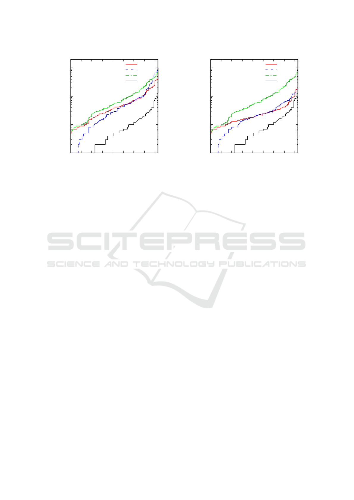
100

1000

0 10 20 30 40 50 60 70 80

Number of validity queries

Number of instances

RPA binary search

RPA multiplying search

git bisect

#inv. leaves

Figure 5: Cumulative distributions of number of performed

validity queries for git bisect and variants of RPA without

propagation. The black line is the cumulative distribution of

number of invalid leaves.

the case of single leaves instances since in this case

the priority queue of RPA fully manifested. Note, that

all plots are in a logarithmic scale.

4.3 Recommendations

We have presented several variants of the RPA algo-

rithm and the experimental results show that the vari-

ants are in general incomparable. There is no variant

that would beat all the others independently of the com-

parison criteria. In the case where the user searches

for a regression predecessor of a single invalid leaf it

makes no sense to use propagation. If the user prefers

ﬁnding the closest regression points, we suggest her

to use multiplying search. In the other case, where

the user rather prefers to minimize the number of per-

formed validity queries, the choice of algorithm de-

pends on the size of the commit graph and also on the

(assumed) distance of regression points from the leaf.

For large commit graphs with no assumptions about

position of regression points we suggest the user to

use RPA with binary search since it guarantees that

only logarithmically many validity queries will be per-

formed. For small commit graphs or graphs where

regression points are assumed to be relatively close to

leaves, we suggest the user to use RPA combined with

multiplying search.

In the other case, where the user searches for re-

gression predecessors of several invalid leaves, it might

be worth to use propagation. If the user prefers ﬁnding

the closest regression points to minimizing the number

of performed validity queries, we suggest her not to

use regression point propagation and employ multiply-

100

1000

0 10 20 30 40 50 60 70 80

Number of validity queries

Number of instances

RPA binary search

RPA multiplying search

git bisect

#inv. leaves

Figure 6: Cumulative distributions of number of performed

validity queries for git bisect and variants of RPA with prop-

agation. The black line is the cumulative distribution of

number of invalid leaves.

ing search. In the opposite case, when the user focus

mainly on minimizing the number of validity queries,

we suggest her to use regression point propagation

and employ either binary search or multiplying search

(based on the size of the commit graph and assumed

positions of regression points as discussed above).

5 CONCLUSION

We have presented a new algorithm, called the Re-

gression Predecessors Algorithm (RPA), for ﬁnding re-

gression points in projects under version control. The

algorithm has several variants, the choice of which

depends on whether the user prefers to minimise the

number of performed validity queries or to ﬁnd the

latest regression points. We have experimentally com-

pared the variants among themselves as well as against

the state-of-the-art tool git bisect. The results show

that the variants of RPA are in general incomparable

as there is no variant that would beat all the others in-

dependently of the criteria. The main strength of RPA

lies in the ability to minimise the number of validity

queries while respecting the requirement to ﬁnd the

latest regression point. In all cases the RPA algorithm

is superior to the algorithm used in git bisect.

ACKNOWLEDGEMENT

This project has received funding from the Elec-

tronic Component Systems for European Leadership

ICSOFT 2018 - 13th International Conference on Software Technologies

162

Joint Undertaking under grant agreement No 692474,

project name AMASS. This Joint Undertaking receives

support from the European Union’s Horizon 2020 re-

search and innovation programme and Spain, Czech

Republic, Germany, Sweden, Austria, Italy, United

Kingdom, France.

REFERENCES

Agrawal, H., Horgan, J. R., Krauser, E. W., and London, S.

(1993). Incremental regression testing. In ICSM, pages

348–357. IEEE Computer Society.

ArangoDB (2018). ArangoDB. https://github.com/arangodb/

arangodb. Accessed: 2018-04-03.

achle, M. and Kirchberg, P. (2007). Ruby on rails. IEEE

Software, 24(6):105–108.

Bazaar (2018). Bazaar. http://bazaar.canonical.com/. Ac-

cessed: 2018-04-03.

Bend

ık, J., Benes, N., Barnat, J., and Cern

a, I. (2016). Find-

ing boundary elements in ordered sets with application

to safety and requirements analysis. In SEFM, volume

9763 of Lecture Notes in Computer Science, pages

121–136. Springer.

Clarke, E. M., Grumberg, O., and Peled, D. A. (2001). Model

checking. MIT Press.

Cormen, T. H., Leiserson, C. E., Rivest, R. L., and Stein, C.

(2009). Introduction to Algorithms (3. ed.). MIT Press.

Duvall, P. M. (2007). Continuous integration. Pearson

Education India.

Git (2018). Git. https://git-scm.com/. Accessed: 2018-04-03.

Git bisect algorithm overview (2018). Git bisect algo-

rithm overview. https://git-scm.com/docs/git-bisect-

lk2009.html. Accessed: 2017-04-03.

Git bisect documentation (2018). Git bisect documentation.

https://git-scm.com/docs/git-bisect. Accessed: 2018-

04-03.

Github Showcases (2018). GitHub Showcases. https://github.

com/showcases. Accessed: 2018-04-03.

Jungnickel, D. (1999). Graphs, networks and algorithms,

volume 5 of algorithms and computation in mathemat-

ics.

Kim, S., Zimmermann, T., Pan, K., and Jr., E. J. W. (2006).

Automatic identiﬁcation of bug-introducing changes.

In ASE, pages 81–90. IEEE Computer Society.

Mercurial (2018). Mercurial. https://www.mercurial-

scm.org/. Accessed: 2018-04-03.

PHP interpreter (2018). PHP interpreter. https://github.com/

php/php-src. Accessed: 2018-04-03.

Pilato, C. M., Collins-Sussman, B., and Fitzpatrick, B. W.

(2008). Version control with subversion - the standard

in open source version control. O’Reilly.

Ruby on Rails (2018). Ruby on Rails. https://github.com/

rails/rails. Accessed: 2018-04-03.

Sliwerski, J., Zimmermann, T., and Zeller, A. (2005). When

do changes induce ﬁxes? ACM SIGSOFT Software

Engineering Notes, 30(4):1–5.

Travis CI (2018). Travis CI. https://travis-ci.org/. Accessed:

2018-04-03.

Verma, R. M. (1994). A general method and a master theo-

rem for divide-and-conquer recurrences with applica-

tions. J. Algorithms, 16(1):67–79.

Zeller, A. (1999). Yesterday, my program worked. today, it

does not. why? In ESEC / SIGSOFT FSE, volume 1687

of Lecture Notes in Computer Science, pages 253–267.

Springer.

Ziftci, C. and Ramavajjala, V. (2015). Heuristics for auto-

mated culprit ﬁnding. US Patent 9,176,731.

Finding Regressions in Projects under Version Control Systems

163