Comparison of Linear State Signal Shaping Model Predictive Control
with Classical Concepts for Active Power Filter Design
Kathrin Weihe
1,2
, Carlos Cateriano Y
´
a
˜
nez
1,2
, Georg Pangalos
1
and Gerwald Lichtenberg
2
1
Application Center Power Electronics for Renewable Energy Systems, Fraunhofer Institute for Silicon Technology ISIT,
Steindamm 94, 20099 Hamburg, Germany
2
Faculty Life Sciences, Hamburg University of Applied Sciences, Ulmenliet 20, 21033 Hamburg, Germany
Keywords:
Model Predictive Control, Active Power Filter.
Abstract:
Many power networks are currently under major change processes due to the necessary integration of re-
newable energy sources. This brings the need to include Active Power Filter (APF) as well as controlling
them in an adequate way. New control concepts like Linear State Signal Shaping Model Predictive Con-
trol (LSSS MPC) are specialized for these tasks and complex compared to classical concepts. Simulation
studies show the advantages of LSSS MPC in performance, robustness and Total Harmonic Distortion (THD)
compensation.
1 INTRODUCTION
The amount of higher order harmonics is increasing
in the electrical grid, due to the increasing share of
sources and loads connected via power converters,
(Liang, 2016). Solar panels use switch-mode invert-
ers to feed energy into the grid with switching fre-
quencies of about 20 kHz (Mohan et al., 2003). Even
with such high frequencies a perfect sine wave can
not be generated, i.e. harmonics are introduced. This
holds true not only for sources but also for loads. One
possibility to cope with this problem is to use ac-
tive power filters (APF) to compensate the harmonics,
(Kumar and Mishra, 2016).
Security and reliability aspects have a strong fo-
cus in power grids, such that a test of a new concept
of compensating harmonics is not performed without
substantial evidence of its functionality, e.g. given by
appropriate simulation studies. In this paper, a novel
controller is compared to one of the well established
and commonly used controllers by closed loop simu-
lations within a standard benchmark grid. Since the
focus of the simulation is to analyse the feasibility of
the new controller, the models involved for the grid
are of low complexity, thus enabling an easier analy-
sis of the controller response.
The most established power control theories for
APF reference current generation are: Instanta-
neous Symmetrical Component (ISC), Instantaneous
Reactive Power (IRP) and Synchronous Reference
Frame (SRF). The ISC theory relies on the transfor-
mation of the instantaneous supply voltages and load
currents, that for unbalanced or distorted supply volt-
age conditions refers to the positive sequence compo-
nents of the supply voltage for the calculation of the
reference current components. On the IRP or p-q the-
ory, the Clarke transformation is used for the trans-
lation of the instantaneous supply voltages and load
currents into the α −β frame, where the compensa-
tion currents are generated and then transformed back
for implementation. The SRF or d-q theory relies on
the dq0 transformation for the load currents, which in-
volves the calculation of the phase θ through a phase
locked loop (PLL), that once in the dq0 domain are
used to compute the reference currents, followed by
an inverse transformation (Kumar and Mishra, 2016).
The strategy proposed in this paper relies on a
novel control approach by a Linear State Signal Shap-
ing Model Predictive Control (LSSS MPC) as intro-
duced in (Cateriano Y
´
a
˜
nez et al., 2018). This theory
establishes that if a desired behaviour of a dynami-
cal linear system lies in a linear signal shape class, a
reformulated linear Model Predictive Control (MPC)
can be used to ensure that state signals are driven into
this class.
The simulation analysis in this paper aims to com-
pare this new control concept against the well estab-
lished p-q theory. For this purpose, the paper is struc-
Weihe, K., Yáñez, C., Pangalos, G. and Lichtenberg, G.
Comparison of Linear State Signal Shaping Model Predictive Control with Classical Concepts for Active Power Filter Design.
DOI: 10.5220/0006910401670174
In Proceedings of 8th International Conference on Simulation and Modeling Methodologies, Technologies and Applications (SIMULTECH 2018), pages 167-174
ISBN: 978-989-758-323-0
Copyright © 2018 by SCITEPRESS – Science and Technology Publications, Lda. All rights reserved
167

tured as follows. In section 2 the main features of
the grid model and the reference current generation
principles are presented, whereas in section 3, the two
control approches are introduced. Section 4 presents
the simulation results and analysis. Finally, section 5
gives a summary and draws conclusions from the sim-
ulation study. A recapitulation of MPC as well as
LSSS MPC is given in the Appendix.
2 GRID MODEL
This chapter introduces the models used for the com-
parative simulation of APF control methods. Starting
from a general definition of state space models the
grid model as well as a single phase equivalent rep-
resentation are given. The section is concluded by an
analysis of the disturbance signal.
2.1 State Space Models
The dynamics of a linear system can be represented
by a continuous-time state space model
˙
x(t) = A
c
x(t) + B
c
u(t) , (1)
where the variable t is time, the vector x ∈ R
n
refers to the state, vector, u ∈ R
m
to the in-
put vector, A
c
∈ R
n×n
to the system matrix,
and B
c
∈ R
n×m
to the input matrix.
Introducing fixed sampling times t
s
taken at t = kt
s
for k = 0, 1, 2, . . ., the model (1) can be rewritten as
discrete state space model
x(k + 1) = Ax(k) + Bu(k) , (2)
with appropriate matrices A ∈ R
n×n
and B ∈ R
n×m
.
2.2 System Description
A simulation of a three-phase three-node grid model
consisting of a three-phase diode rectifier acting as
a non-linear load is used to evaluate the proposed
new control method to compensate current harmonics
with. Active power filters can be connected in series
or in parallel (shunt) to the load, with series APF be-
ing suitable for power quality improvement, (Hashim
et al., 2016) while shunt APF are used to provide reac-
tive power and current harmonics compensation, (Ak-
agi, 2005).
Figure 1 shows the electrical circuit configura-
tion of the simulation setup. The grid model uses a
balanced supply of 230 V root mean square (RMS)
phase-to-ground voltage with a frequency of 50 Hz,
hence a shunt configuration for the APF is chosen.
Active filter configurations most commonly consist
of a three-phase voltage-source pulse width modula-
tion converter (VSC) utilizing a DC link capacitor as
voltage supply, a coupling inductor to filter switching
ripples and a controller. The filter detects the instan-
taneous load current i
l
and applies the compensating
current i
f
at the point of common coupling (PCC) to
cancel out harmonics.
V
s
R
f
L
f
i
fC
i
cc
R
c
L
c
V
s
R
f
L
f
i
f B
i
cb
V
s
R
f
L
f
i
f A
i
ca
APF
i
lc
L
l
i
lb
L
l
i
la
L
l
C
DC
R
l
C
DC
R
l
C
DC
R
l
Figure 1: Three-phase three-node grid model.
2.3 Single Phase Equivalent Circuit
The system behaviour can approximately be modelled
as a current source providing non-linear currents to
the grid which leads to the single phase equivalent
circuit shown in Figure 2. The non-linear load is rep-
resented by an uncontrollable current source, the APF
acts as controllable current source, and the supply is
modelled by a voltage source. The non-linear load is
connected to the supply voltage by a feeder line with
the resistance R
f
and the inductance L
f
respectively,
which generate a voltage drop v
l
over the feeder line.
To reduce modelling complexity the LSSS MPC em-
ploys a state space model of the single phase equiva-
lent circuit to calculate the compensation current.
v
s
R
f
L
f
i
f
i
c
i
l
v
1
Figure 2: Single phase equivalent circuit of a shunt active
filter compensating a non-linear load.
The model has the state vector:
x =

v
l
di
c
dt
di
l
dt

|
∈ R
3
(3)
with the control input u(t) =
d
2
i
c
dt
2
∈ R and the distur-
SIMULTECH 2018 - 8th International Conference on Simulation and Modeling Methodologies, Technologies and Applications
168

bance d(t) =
d
2
i
l
dt
2
. The state space model is given as
dx
1
dt
= −R
f
x
2
+ R
f
x
3
−L
f
u(t) + L
f
d(t) (4)
dx
2
dt
= u(t) (5)
dx
3
dt
= d(t) (6)
where (4) can be derived by Kirchhoff’s circuit
laws. In order to gain access to the feeder line volt-
age v
l
as state, an augmented state space model is de-
rived with additional states in (5) and (6). Note, that
this leads to a reformulation of the original input i
c
and disturbance i
l
.
2.4 Disturbance Signal
The non-linear load current i
l
is modelled as an ideal
current source acting as a disturbance d(t) to the sin-
gle phase state space model as shown in figure 2. In
order to generate the disturbance, a physical model
of a diode rectifier is simulated as part of the grid
model shown in figure 1. Due to the nature of the
diodes included, a non-linear current-voltage charac-
teristic can be observed when using a bridge rectifier.
Although methods exist to obtain a state space model
for such devices (Emadi, 2001), simulation tools like
MATLAB SIMULINK have the great advantage of pro-
viding transient analysis of power electronics without
the need to perform the complex modelling process.
In this paper the grid model including the rectifier
is built using SIMULINK models. The current load
drawn by the rectifier is measured and fed in to the
state space model which affects the calculation of the
compensation current generated by the controller, ef-
fectively affecting back the physical model of the rec-
tifier in the grid. Thus the measurement of the distur-
bance is constantly updated by the simulation of the
physical diode rectifier model.
3 CONTROLLER MODELS
To achieve good harmonic compensation, APF need
to detect the harmonic content drawn from the load
in order to inject the inverse equivalent as compen-
sation current into the PCC. Conventional APF use
high pass filter to extract harmonics from the load
current. High performance digital signal processors
(DSPs), field-programmable gate arrays (FPGAs) to-
gether with high precision current and voltage mea-
surement devices need to be utilized to guarantee as
little errors in current detection as possible, as errors
and delays can reduce the performance of the APF or
even evoke instability (Malesani et al., 1998).
In contrast to this, the LSSS MPC does not rely on
a high pass filter but instead uses a linear shape class
defining a fundamental harmonic condition to calcu-
late a compensation current which is able to obtain a
sinusoidal signal, see section 3.2.
3.1 Classical Control for Shunt APF
Among a wide range of methods to calculate the ref-
erence compensation current, the instantaneous active
and reactive power theory (p-q theory) (Akagi et al.,
1986) has proven to provide good harmonic compen-
sation performance both in simulation and application
(Akagi, 2005). The PCC voltages and load currents
are transformed into the α −β orthogonal frame us-
ing the Clarke transformation defined as

v
α
v
β

=
r
2
3

1 −
1
2
−
1
2
0
√
3
2
−
√
3
2



v
f A
v
f B
v
fC


(7)

i
lα
i
lβ

=
r
2
3

1 −
1
2
−
1
2
0
√
3
2
−
√
3
2



i
lA
i
lB
i
lC


. (8)
The instantaneous real power p
l
and instantaneous
imaginary power q
l
are then calculated by

p
l
q
l

=

v
α
v
β
−v
β
v
α

i
lα
i
lβ

. (9)
Assuming a purely sinusoidal source voltage, both p
l
and q
l
can be separated into a DC and an AC com-
ponent with the previous mentioned high pass filter,
with the AC component referring to the amount of
harmonic distortion incorporated in the load current.
The reference compensation current i
c,re f
is generated
by applying the inverse Clarke transformation to the
AC component of p
l
and q
l
.
To induce the compensation current into the grid,
a VSC controlled by a hysteresis band controller is
used in this paper. The switching signals are gener-
ated by comparing the compensating current i
c
with
the reference current i
c,re f
and calculating the cur-
rent error. If the error exceeds the upper or lower
limit of a fixed hysteresis band, the legs of the VSC
are switched accordingly, so the compensating current
stays inside the hysteresis band (Buso et al., 1998).
It is worth mentioning, that while simple in im-
plementation and robust in application, the hystere-
sis band controller produces varying switching fre-
quencies, which can lead to unsatisfactory behaviour
(Buso et al., 1998).
Comparison of Linear State Signal Shaping Model Predictive Control with Classical Concepts for Active Power Filter Design
169

3.2 New Shape Class MPC Controller
The control focus of the APF of this implementation
is the compensation of the THD on the feeder cur-
rent i
f
and the feeder voltage v
f
, i.e leading them
into the shape class of perfect fundamental harmonic
functions. The property of this shape class can be ex-
pressed as the solution of the initial value problem of
the homogeneous ordinary second order differential
equation (ODE)
d
2
x(t)
dt
2
+ (2π f )
2
x(t) = 0, (10)
that leads to a sinusoidal state signal x(t) with a
fixed frequency f , zero offset, and an arbitrary am-
plitude, (Ahlfors, 1966).
In order to express the ODE in (10) as a linear
shape class of the form (19) as given in the appendix,
it needs to first be transformed into a discrete-time
form. This can be achieved using forward numer-
ical differentiation to approximate the second order
derivative in (10), with a step size t
s
and an accuracy
order of O(t
2
s
), (Fornberg, 1988),
d
2
x(t)
dt
2
≈
2x(k) −5x(k + 1) + 4x(k + 2) −x(k + 3)
t
2
s
,
(11)
that when replaced in (10) starting at discrete
time k + 1 (first future time step), leads to a linear
shape class with s = 1, n = 1, and T = 4, defined by
the row vector
v =
1
t
2
2

2 + (2π f t
s
)
2
5 4 −1

∈ R
1×4
. (12)
Note that by using forward numerical differentiation
the signal shape can be expressed by only using future
state predictions which results in a homogeneous set-
up for the Q weight matrix, while using a more pre-
cise centered approximation would require to modify
the prediction horizon to include past states.
4 SIMULATION STUDIES
MATLAB SIMULINK is used to simulate the model in
order to evaluate the performance and feasibility of
the LSSS MPC method compared to the IRP method.
4.1 Parameter Settings
The simulation is run with a fixed-step solver with dif-
ferent fundamental sample times for the IRP APF and
the LSSS MPC as explained in greater detail in sec-
tion 4.2. Simulations showed that a first order Eu-
ler forward solver provides sufficient accuracy and is
chosen over a higher order solver to improve simula-
tion speed.
Table 1: Simulation parameters.
Parameter Symbol Value
Sampling time IRP APF t
s1
1 ×10
−6
s
Sampling time MPC APF t
s2
2 ×10
−5
s
Phase-to-ground RMS voltage v
s
230 V
Grid frequency f 50 Hz
Feeder line resistance R
f
1 Ω
Feeder line inductance L
f
0.01 mH
Filter coupling resistance R
c
0.001 Ω
Filter coupling inductance L
c
3.50 mH
VSC DC Link voltage V
DC
700 V
AC load coupling inductance L
l
2 mH
DC smoothing capacitor C
DC
0.68 mF
Table 1 shows the parameters of the grid model.
A bridge rectifier using a smoothing capacitor on the
DC side is connected to every phase of the grid model,
drawing non-linear currents. To analyse different load
scenarios and transient behaviour of the APF, three
different load steps are implemented. Starting from
a 100 Ω resistance at the DC side of the rectifier, after
a simulation time of 0.3 s the load resistance drops
to 9 Ω and after a simulation time of 0.6 s to 2 Ω
respectively to simulate an increase in load current
drawn from the grid. The high pass filter for the clas-
sical IRP APF is designed using standard methods
(Akagi et al., 1986). The DC link voltage of the VSC
used to generate compensation currents is controlled
by a PI-Controller that was tuned using the Ziegler-
Nichols method (Ziegler and Nichols, 1942). Addi-
tionally, in order to enable the IRP APF to react on
time to the changes in load current of the rectifier, an
AC load coupling inductance L
l
is needed in series be-
tween the rectifier and the PCC; this limitation is not
present on the LSSS MPC, howerever is also included
for simulation consistency.
The Q and R matrices are tuned heuristically, with
the cost of control effort tuned to 8 ×10
3
, the cost
of control error is presented in table 2. Only the
weight for the feeder line voltage is set to ensure a
Table 2: Q matrix tuning.
State State weight
v
l
10
3
di
c
dt
0
di
l
dt
0
SIMULTECH 2018 - 8th International Conference on Simulation and Modeling Methodologies, Technologies and Applications
170

sinsudoidal signal shape, assuming this can only be
achieved by sinusoidal feeder line current. The length
of prediction horizon H
p
and input horizon H
u
are
chosen to be equal to the number of samples in one
period
1
f t
s2
. The controller updates once per period, in
contrast to traditional MPC which updates once per
sample. This means that the controller uses its full
predicted optimal input and not only the first value as
usual with the MPC. This update setup is chosen in
accordance with the periodic behaviour of the target
fundamental harmonic shape class.
4.2 Assumptions and Criteria
The LSSS MPC incorporates a model of the sin-
gle phase equivalent circuit, so the controller is able
to calculate the compensation current for one phase
only. Both APF are connected to the three-phase
three-node model, with the LSSS MPC being capa-
ble of providing compensation for one phase in the
current state of development. To provide a compara-
ble performance evaluation, the simulation results for
one phase will be presented.
Also note, that an APF utilizing a hysteresis band
controlled VSC is a source of harmonic currents itself
by inducing the compensation current with a variable
switching frequency. On the other hand, the LSSS
MPC uses an ideal current source to generate the com-
pensation current for the benefit of reduced modelling
complexity. To provide an environment, where addi-
tional harmonic distortion due to the switching ripples
of the VSC is minimized, a high sampling frequency
of 100 kHz is chosen for the simulation of the IRP
APF method as well as small upper and lower band
limits of 0.01 A for the hysteresis controller.
In order to analyse the compensation perfor-
mance, the total harmonic distortion THD is calcu-
lated by
THD =
p
∑
∞
n=2
X
2
n
X
1
, (13)
where THD refers to the ratio of the RMS values of
higher order harmonic frequencies X
n
to the funda-
mental X
1
, (Shmilovitz, 2005).
4.3 Results
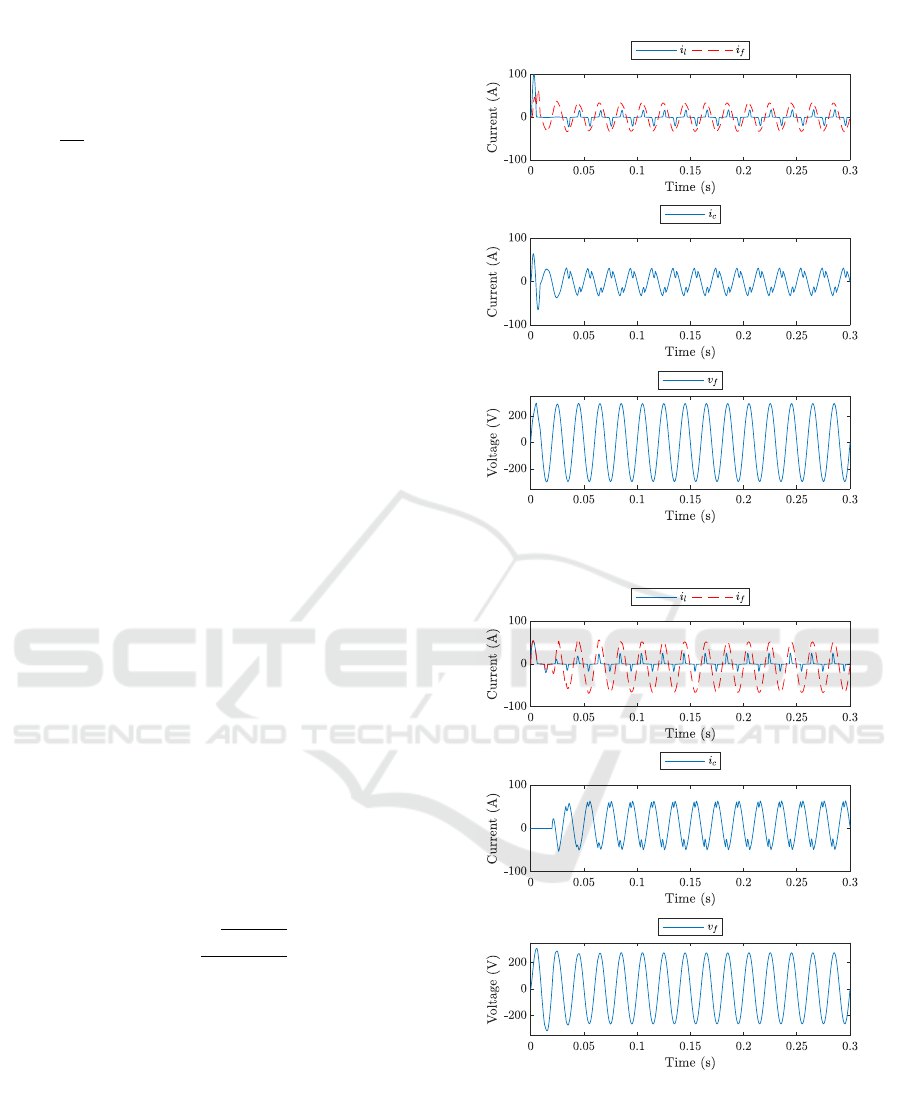
As can be seen in figure 3 the classical APF using the
IRP method generates a compensation current (mid
plot) which leads to a nearly purely sinusoidal feeder
line voltage (bottom plot) and current (top plot, red
dashed line).
Similar results can be observed for the APF us-
ing the LSSS MPC, as shown in figure 4. However, a
Figure 3: Simulation results for the load compensation us-
ing IRP APF.
Figure 4: Simulation results for the load compensation us-
ing LSSS MPC APF.
higher amplitude in the compensation current can be
observed from the mid plot which can be interpreted
as an excess of energy going into the load current (top
plot, blue solid line). Also note, that there is a DC off-
set in the feeder current, which dissipates with longer
simulation time and higher amount of harmonic dis-
tortion.
Comparison of Linear State Signal Shaping Model Predictive Control with Classical Concepts for Active Power Filter Design
171

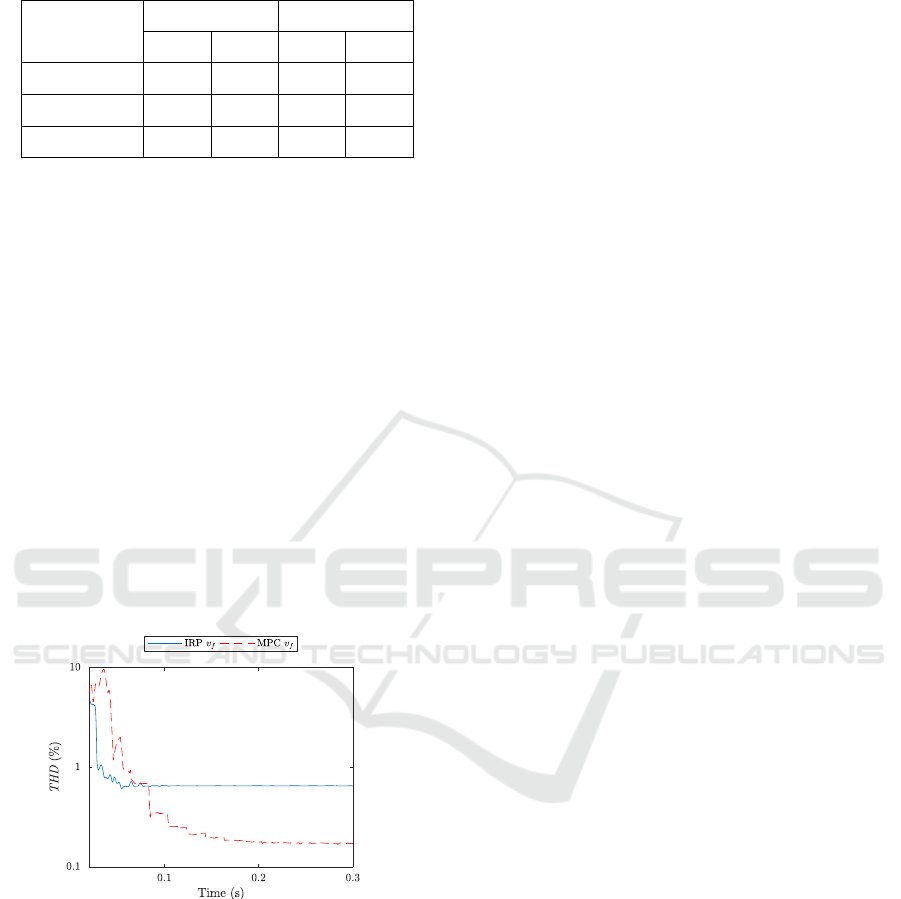
Table 3: Simulation results for THD reduction of feeder line
voltage and current.
Load scenario
THD (v
f
) THD (i
f
)
IRP MPC IRP MPC
100 Ω 0.65% 0.17% 4.35% 0.78%
9 Ω 0.45% 0.35% 0.75% 1.57%
2 Ω 1.15% 0.35% 3.75% 1.33%
Figure 5 shows the evolution of the feeder line
voltage THD for the first load step for both compensa-
tion methods. While the IRP APF settles to a THD of
0.65% after around 0.05 s, the LSSS MPC continues
to reduce the THD to 0.17%.
Table 3 shows the simulation results for the feeder
line voltage and current THD reduction for the whole
simulation time frame including the three different
load scenarios. The LSSS MPC APF achieves bet-
ter overall THD reduction of the feeder line volt-
age and current, adapting to the different load step
changes. However, the IRP APF shows a better re-
sult for the feeder current only in the second load step
scenario for which the AC load coupling inductance
was specifically parametrized. It is important to no-
tice that the LSSS MPC was only implicitly tuned to
compensate the feeder voltage, which can explain its
overall better performance on voltage against current
THD.
Figure 5: Dynamic behaviour of the THD reduction for the
first load scenario.
5 CONCLUSIONS
This section summarises the paper and gives an out-
look on future work.
5.1 Summary
A simulation testbench has been built to compare a
novel LSSS MPC control method to a classical IRP
APF approach. While the high pass filter on an IRP
APF needs to be specifically designed to work in a
given load scenario, the LSSS MPC through its cost
function is capable of adapting to a wider variety of
load scenarios. The simulation results show that an
LSSS MPC approach has the potential to success-
fully control an APF. Since the LSSS MPC consid-
ers predictions of the disturbance one period ahead, it
is more flexible to adapt to abrupt load changes, thus
not actually needing an AC load coupling inductance
which is the case for the IRP APF.
5.2 Outlook
While the LSSS MPC shows good overall compensa-
tion results in the simulated time frame, the observed
excess in compensation current should be avoided to
minimize the energy consumption of the APF. For
longer simulation time the excess of energy can even
keep building up. This can be addressed by apply-
ing a state constraint to the LSSS MPC, however this
could lead to a higher computational effort. Addition-
ally, to control both feeder line voltage and current,
the cost function of the LSSS MPC would need to be
adapted to penalize both states, thus leading to a more
challenging tuning of the Q and R matrices. Apply-
ing constraints to the LSSS MPC as well as tuning the
controller under more complex conditions is currently
being researched.
ACKNOWLEDGEMENTS
This contribution was partly developed within the
project NEW 4.0 (North German Energy Transition
4.0) which is funded by the German Federal Ministry
for Economic Affairs and Energy (BMWI). This pa-
per was also partly funded by the Free and Hanseatic
City of Hamburg (Hamburg City Parliament publica-
tion 20/11568).
REFERENCES
Ahlfors, L. (1966). Complex Analysis: An introduction to
the theory of analytic functions of one complex vari-
able. Harvard University.
Akagi, H. (2005). Active Harmonic Filters. Proceedings of
the IEEE, 93(12):2128–2141.
SIMULTECH 2018 - 8th International Conference on Simulation and Modeling Methodologies, Technologies and Applications
172

Akagi, H., Nabae, A., and Atoh, S. (1986). Control Strat-
egy of Active Power Filters Using Multiple Voltage-
Source PWM Converters. IEEE Transactions on In-
dustry Applications, IA-22(3):460–465.
Buso, S., Malesani, L., and Mattavelli, P. (1998). Com-
parison of current control techniques for active filter
applications. IEEE Transactions on Industrial Elec-
tronics, 45(5):722–729.
Cateriano Y
´
a
˜
nez, C., Pangalos, G., and Lichtenberg, G.
(2018). An approach to linear state signal shaping by
quadratic model predictive control. In 2018 European
Control Conference (ECC). Accepted.
Emadi, A. (2001). Modelling of power electronic loads in ac
distribution systems using the generalized state space
averaging method. In Industrial Electronics Society,
2001. IECON ’01. The 27th Annual Conference of the
IEEE, volume 2, pages 1008–1014 vol.2.
Fornberg, B. (1988). Generation of finite difference formu-
las on arbitrarily spaced grids. Mathematics of com-
putation, 51(184):699–706.
Hashim, H. F., Omar, R., and Rasheed, M. (2016). De-
sign and analysis of a three phase series active power
filter (SAPF) based on hysteresis controller. In 4th
IET Clean Energy and Technology Conference (CEAT
2016), pages 1–5.
Kumar, P. and Mishra, M. K. (2016). A comparative study
of control theories for realizing APFs in distribution
power systems. In 2016 National Power Systems Con-
ference (NPSC), pages 1–6.
Liang, X. (2016). Emerging power quality challenges due to
integration of renewable energy sources. IEEE Trans-
actions on Industry Applications, PP(99):1–1.
Maciejowski, J. (2001). Predictive control with constraints.
Hemel Hempsted: Prentice Hall/ Pearson Education.
Malesani, L., Mattavelli, P., and Buso, S. (1998). On the
applications of active filters to generic loads. In 8th
International Conference on Harmonics and Quality
of Power. Proceedings (Cat. No.98EX227), volume 1,
pages 310–319 vol.1.
Mohan, N., Undeland, T. M., and Robbins, W. P. (2003).
Power Electronics. Converters, Applications and De-
sign. John Wiley and Sons, Inc, third edition.
Shmilovitz, D. (2005). On the definition of total har-
monic distortion and its effect on measurement in-
terpretation. IEEE Transactions on Power Delivery,
20(1):526–528.
Ziegler, J. G. and Nichols, N. B. (1942). Optimum settings
for automatic controllers. Transactions of the ASME,
64:759768.
APPENDIX
Model Predictive Control (MPC)
Following the state space dynamics in (2), consid-
ering the state reference vector r ∈ R
n
, the predic-
tion horizon H
p
∈ N and the input horizon H
u
∈ N,
the MPC standard quadratic cost function can be for-
mulated, (Maciejowski, 2001)
J(k) = kX(k) −Ξ(k)k
2
Q
+ k∆U(k)k
2
R
(14)
for the optimization problem
min
∆U(k)
J(k), (15)
where X(k) ∈ R
H
p
n
is the future state sequence
prediction, Ξ(k) ∈ R
H
p
n
the future reference trajec-
tory, and ∆U(k) ∈ R
(H
u
+1)m
the control input change
sequence. Considering with the cost of con-
trol error given by the positive semi-definite ma-
trix Q ∈ R
H
p
n×H
p
n
and the cost of control effort by
the positive definite matrix R ∈ R
(H
u
+1)m×(H
u
+1)m
.
The solution of (15) is given by the optimal con-
trol input sequence ∆U
?
(k), which is fed to the plant,
as shown in the standard MPC control loop of Fig-
ure 6.
Controller
Optimization
Prediction
Model
Plant
u
x
r
Figure 6: Model Predictive Controller: Classical Scheme.
In order to find the solution ∆U
?
(k) in the uncon-
strained scenario in a numerically well-conditioned
manner, the cost function J(k) can be rearranged as
J(k) =





S
Q
(X(k) −Ξ(k))
S
R
∆U(k)





2
, (16)
with the cost matrices factorization
Q = S
Q
|
S
Q
, (17)
R = S
R
|
S
R
, (18)
which can be efficiently solved in the least-square
sense, e.g. using a QR algorithm, leading to a linear
time invariant system controller (Maciejowski, 2001).
Typically the MPC controller uses the receding
horizon principle to set an update time strategy for the
controlled input signal, where only the first element of
the computed optimal input vector sequence ∆U
?
(k)
is given to the system, then the state values are mea-
sured or observed, resp., (Maciejowski, 2001).
Comparison of Linear State Signal Shaping Model Predictive Control with Classical Concepts for Active Power Filter Design
173

Linear State Signal Shaping MPC
A linear shape class of a discrete-time state vector
signal can be formulated as a kernel representation set
X
V
=
{
x(1), x(2), . . .
|
V



x(k + 1)
.
.
.
x(k + T )



=0 ∀k = 0, 1, . . .
}
, (19)
where the matrix V ∈R
s×nT
defines the behaviour
of the state signal shape class, (Cateriano Y
´
a
˜
nez et al.,
2018).
If a desired behaviour of a dynamical linear sys-
tem lies in a special signal shape class given by its
kernel representation (19), a control algorithm which
ensures that state signals are driven to this class be-
longs to the class of linear MPC problems, (Cateriano
Y
´
a
˜
nez et al., 2018).
This can be achieved as follows. For H
p
≥ T ,
let V
j
= V
:,( j−1)n+1: jn
, the band matrix
P
V
=







V
1
V
2
··· V
T
0 ··· 0
0 V
1
V
2
··· V
T
.
.
.
.
.
.
.
.
.
.
.
.
.
.
.
.
.
.
.
.
.
.
.
.
0
0 ··· 0 V
1
V
2
··· V
T







∈R
p
1
×p
2
, (20)
with p
1
= s(H
p
−T + 1) and p
2
= nH
p
, can be
computed by shifting the shape class matrix V of (19)
for integer multiples of n columns with the help of
matrices of zeros 0 = {0}
s×n
.
Remark: For H
p
= T , the matrix P
V
= V is trivial.
The solution of the MPC optimization prob-
lem (15) with reference Ξ(k) = 0, weighting ma-
trices R = 0, and Q = P
V
|
P
V
, leads the state se-
quence x(k + 1), x(k + 2), . . . in the shape class given
by the matrix V, (Cateriano Y
´
a
˜
nez et al., 2018).
Remark: For R 6= 0, The minimum J(k) will rely
on a trade off between the cost of control effort intro-
duced by R and the original cost of control error of
not being in the shape class (Cateriano Y
´
a
˜
nez et al.,
2018).
SIMULTECH 2018 - 8th International Conference on Simulation and Modeling Methodologies, Technologies and Applications
174