Dow Jones Trading with Deep Learning: The Unreasonable Effectiveness

of Recurrent Neural Networks

Mirco Fabbri and Gianluca Moro

Department of Computer Science and Engineering (DISI), University of Bologna,

Via Cesare Pavese, I-47522, Cesena, Italy

Keywords:

Stock Market Prediction, Trading, Dow Jones, Quantitative Finance, Deep Learning, Recurrent Neural

Network, LSTM.

Abstract:

Though recurrent neural networks (RNN) outperform traditional machine learning algorithms in the detection

of long-term dependencies among the training instances, such as in term sequences in sentences or among

values in time series, surprisingly few studies so far have deployed concrete solutions with RNNs for the stock

market trading. Presumably the current difﬁculties of training RNNs have contributed to discourage their wide

adoption.This work presents a simple but effective solution, based on a deep RNN, whose gains in trading with

Dow Jones Industrial Average (DJIA) outperform the state-of-the-art, moreover the gain is 50% higher than

that produced by similar feed forward deep neural networks. The trading actions are driven by the predictions

of the price movements of DJIA, using simply its publicly available historical series. To improve the reliability

of results with respect to the literature, we have experimented the approach on a long consecutive period of

18 years of historical DJIA series, from 2000 to 2017. In 8 years of trading in the test set period from 2009 to

2017, the solution has quintupled the initial capital, moreover since DJIA has on average an increasing trend,

we also tested the approach with a decreasing averagely trend by simply inverting the same historical series

of DJIA. In this extreme case, in which hardly any investor would risk money, the approach has more than

doubled the initial capital.

1 INTRODUCTION

Past stock market prediction approaches, which were

based on analysis of macroeconomic variables, led

to the formulation of Efﬁcient Market Hypothesis

(EMH) (Fama, 1970) according to which the ﬁnancial

market is efﬁcient and reﬂects not only the informa-

tion publicly available (e.g. news, stock prices etc.)

but also the future expectations of traders. This re-

sult, together with the study in (Malkiel, 1973) that

showed accordance between the stock values and the

random walk theory, corroborate the idea of the stock

market unpredictability.

Despite these outcomes, the literature in stock

market predictions is among the most long-lived rese-

arches, evidently in the attempt of rejecting the hypot-

hesis of the market unpredictability, such as in (Lo

and MacKinlay, 1988) and in (Malkiel, 2003) where,

being random walk theory conﬁrmed only within a

short time window, the market trend should generally

be predictable. The last two mentioned studies do not

contradict the EMH because the possibility of pre-

dicting the stock prices trend is not necessarily linked

to the market inefﬁciency but to the predictability of

the ﬁnancial macro variables.

As we have more extensively reported in Section

2, the stock prediction methods have ranged from

auto-regressive ARIMA models (Box and Jenkins,

1970) to more advanced approaches also based on

machine learning, including in the last decade the

neural networks, using both structured and unstruc-

tured data, namely time series and free text such as

news, posts, forums etc. (Mitra, 2009; Atsalakis and

Valavanis, 2009a; Mostafa, 2010).

The novel proposals, which have improved the

accuracy predictions of preceding approaches, are ba-

sed on the combination of time series values with

news or social network posts, such as in (Bollen et al.,

2011; Domeniconi et al., 2017a; Akita et al., 2016).

The drawback of combining ﬁnancial time series and

news or posts, is that such approaches require daily

huge amount of fresh text which are almost impossi-

ble to gather in real time, even because the sources

of news and social networks do not permit like in the

142

Fabbri, M. and Moro, G.

Dow Jones Trading with Deep Learning: The Unreasonable Effectiveness of Recurrent Neural Networks.

DOI: 10.5220/0006922101420153

In Proceedings of the 7th International Conference on Data Science, Technology and Applications (DATA 2018), pages 142-153

ISBN: 978-989-758-318-6

past unconditional massive download of their data. In

other words their application appear unfeasible in real

time scenarios typical of the stock market exchange.

Recently the deep learning has become a wide

and proliﬁc area of research with successful bre-

akthroughs in several scientiﬁc and business areas,

such as speech and image recognition (Krizhevsky

et al., 2012), autonomous driving, diagnosis of dise-

ases or genomic bioinformatics (Esteva et al., 2017;

Domeniconi et al., 2016; di Lena et al., 2015), as-

tronomical discoveries and so on. The impressive ef-

fectiveness of deep learning solutions rely on novel

neural networks with memory capabilities. In particu-

lar recurrent neural networks (RNN) are the ﬁrst con-

crete learning technology capable of detecting long-

term dependencies among the training instances, such

as among consecutive words in sentences (Domeni-

coni et al., 2017b) or among consecutive values in

time series.

Despite this capability of detecting temporal cor-

relations or patterns, surprisingly few studies so far

have deployed concrete solutions with for the stock

market trading based on RNNs. One of the main rea-

sons that have limited the wide employment of RNNs

for predicting the stock market, is that deﬁning and

training a successful RNN is almost always a chal-

lenge. In fact the number of choices to discover an

effective RNN, are much more large and mutually

dependent with respect to the preceding approaches:

concretely the choices start from the architecture de-

sign, such as the number of neuronal layers, the neu-

ronal units in each layer, the number of connections

among layers, the kind of activation functions in each

neuron unit and so on, up to the discovery at training

time from a wide number of hyper-parameters, those

that maximise the test set accuracy.

The contribution of this work is the set of the

successful choices that have led to the deﬁnition, im-

plementation and training of a deep RNN for trading

with the Dow Jones Industrial Average (DJIA), whose

proﬁts outperform the state-of-the-art. The solution

is also a trade-off among efﬁcacy and efﬁciency in

order to be applied in real time trading and there-

fore using only publicly available historical series of

DJIA, without any further external data. The solu-

tion performs trading actions, such as buy/sell/none,

from the ability of predicting accurately the closing

price movements of DJIA, which appears unreasona-

ble being in contradiction with the stock market un-

predictability.

Our approach has quintupled the initial capital in

the test phase of the last 8 years of trading, between

2010 and 2017, after a training phase between 2000

http://tiny.cc/dow jones trading

and 2009. The proﬁt is about 50% higher than achie-

vable via a Feed-Forward (FF) deep neural network,

which is without explicit memory capacity. The DJIA

has on average a positive trend and to evaluate the ro-

bustness of our solution, we have applied it also to the

historically inverted DJIA, which consequently is on

average a negative time series. In this extreme case,

where investors would not risk money, the gain pro-

duced is 2.33 times the initial capital.

The study is organised as follows. Section 2 ana-

lyses the recent literature in the stock market pre-

diction, from classical methods to those based on

news and on social network posts. Section 3 des-

cribes the data set employed and the proposed solu-

tion with a brief background on recurrent neural net-

works. Section 4 reports the experiment results and

how they outperform preceding results with DJIA ba-

sed on neural networks. Section 5 summarises the

work and outlines the future developments.

2 RELATED WORKS

The literature of stock market predictions is large

being a long time research thread that goes from clas-

sic historical series forecasting to social media analy-

sis.

A well-known research in (LeBaron et al., 1999),

in contrast to the unpredictability of the stock market,

explains the existence of a temporal lag between the

issuance of new public information and the decisions

taken by the traders. In this short time frame the new

information can be used to anticipate the market.

In 2009 (Schumaker and Chen, 2009), following

this idea that new information may quickly inﬂuence

the trading, experimented the prediction of stock pri-

ces by combining ﬁnancial news with stock prices

through Support Vector Machine (SVM). They tried

to estimate the stock price 20 minutes after the rele-

ase of the new information achieving actually the best

results with the combination of text news and stock

values.

Successively other works proposed methods that

combine the text mining techniques with data mining

techniques. (Lin et al., 2011) combines K-means and

hierarchical clustering to analyse ﬁnancial report (for-

mal record of the ﬁnancial activities and position of a

business, person, or other entity (Wikipedia contribu-

tors, 2018)) through quantitative and qualitative featu-

res. This approach allows to detect clusters of features

and improves the quality of prototypes of the reports.

The most prominent approach used in time-series

forecasting has been introduced in 1970 by Box and

Jenkins and it is called ARIMA (Autoregressive inte-

Dow Jones Trading with Deep Learning: The Unreasonable Effectiveness of Recurrent Neural Networks

143

grated moving average (Box and Jenkins, 1970)); it

shows an effective capability to generate short-term

forecasts. ARIMA considers future values as linear

combination of past values and past errors, expressed

as follows:

= φ

+ φ

t−1

+ φ

t−2

+ . . . φ

t− p

. . .

+ε

− θ

t−1

− θ

t−2

− θ

t−q

(1)

where Y

is the actual stock value, ε

is the random er-

ror at time t, φ

and θ

are the coefﬁcients and p, q are

integers called autoregressive and moving average.

The main advantage of this approach, is the ability of

observing it from two perspectives: statistical and ar-

tiﬁcial intelligence techniques. In particular ARIMA

methodology is known to be more efﬁcient in ﬁnan-

cial time series forecasting than ANNs (Lee et al.,

2007; Merh et al., 2010; Sterba and Hilovska, 2010).

Some works that used ARIMA are (Khashei et al.,

2009; Lee and Ko, 2011; Khashei et al., 2012).

Recent studies as (Lo and Repin, 2002) in behavi-

oural ﬁnance and behavioural economy have applied

cognitive psychology in order to understand the re-

asons that led investors to make certain choices and

how these affect the market trend. This, together with

ability of computers to process massive amounts of

data, has given a strong boost to a research thread

which tries to correlate the sentiment acquired from

repositories of social opinion (as social media or jour-

nalistic news) to the market trend. Some of these stu-

dies use mining technique to predict stock prices (e.g.

the DJIA) (Gidofalvi and Elkan, 2001), (Schumaker

and Chen, 2006), or to make more accurate predicti-

ons detecting relevant tweets such as in (Domeniconi

et al., 2017a). Furthermore, signiﬁcant steps taken

in natural language understanding (NLU) and natural

language processing (NLP) achieved a new state-of-

the-art in the ﬁeld of market forecasting by exploi-

ting deep neural networks (Akita et al., 2016; Wang

et al., 2017; Fisher et al., 2016). The idea behind the

use of NLP lies in the ability of extracting sentiments

and opinions directly from unstructured data and ex-

ploits them to predict market trend. (Tetlock, 2007)

has analysed the correlation between sentiment, ex-

tracted from news articles, and the market price trend

with the conclusion that media pessimism may affect

both market prices and trading volume.

Similarly (Bollen et al., 2011; Domeniconi et al.,

2017a) have taken advantage of text mining techni-

ques to extract mood from social media, like Twitter,

and improve the DJIA index prediction; in both cases,

the result obtained are very interesting because they

achieved an accuracy of 86% and 88% respectively.

Another consideration can be raised from Bollen et

al. work relative to the time-lag. Their study showed

that the best performance can be obtained grouping

information from several past days to predict the next

one.

Also in the deep learning thread, NLP methods

have been used to improve language understanding

and tackle ﬁnancial market trading. (Akita et al.,

2016) experiments the possibility of predicting stock

values by exploiting existing information correlations

between companies. For every day predictions, the

set of news related to companies is converted in a dis-

tributed representation of features by using Paragraph

Vector which is then used to feed a memory network

along with stock prices. Then the model is trained

to predict the output class, buy if the predicted close

price is greater than real opening prices, otherwise

sell.

(Ding et al., 2015) introduces a new techni-

que, which proposes to automatically extract a dense

representation of event embeddings from ﬁnancial

news. To do that, a word embedding approach is used

to create a distributed representation of words, taken

from Reuters and Bloomberg news, and used to feed

a Neural Tensor Network (NTN) subsequently produ-

cing a distributed representation of event embeddings.

These events are used to feed common models like FF

or convolutional neural networks. The prediction has

been done on S&P 500 stock and it showed an accu-

racy of 65% and an economical proﬁt of 1.68 times

the initial capital.

However, the works that use NLP and NLU to pre-

dict market movements are de facto inapplicable in

real time scenarios because they should continuously

collect and process large amounts of fresh, noise-free

unstructured textual data from sources, such as Web

news sites and social networks, which now, further-

more, prevent unconditional and massive data gather-

ing.

There are, however, several studies that have em-

ployed neural network to forecast stock market using

only structured data such as time series or ﬁnancial

data (Atsalakis and Valavanis, 2009b; Soni, 2011).

(Olson and Mossman, 2003) attempted to predict

annual stock returns for 2352 Canadian companies

by feeding a neural network with 61 accounting re-

ports obtaining better results than those obtained by

regression-based methods. Similarly (Cao et al.,

2005) has shown that neural networks outperformed

the accuracy predictions of generalised linear models

in Chinese stock market.

Although neural networks have provided good re-

sults in stock market forecasting, they do not achieve

the same performance achievable through Deep Lear-

ning, as reported in (Abe and Nakayama, 2018). In

this work different models of both shallow and FF

deep neural networks are compared; they are fed by

DATA 2018 - 7th International Conference on Data Science, Technology and Applications

144

the combination of market and ﬁnancial data to pre-

dict one-month-ahead stock returns of MSCI Japan

Index.

In (Fischer and Krauss, 2017) LSTM networks

have been compared with classical methods, among

which Random Forest, for the prediction of the S&P

500 (Thomson Reuters) between the years 1993 and

2015. They have obtained an unstable effectiveness

with signiﬁcant differences in the following three pha-

ses:

• 1993-2000: The cumulative proﬁt at the end of

this period was about 11 times the initial capital,

also overcoming the random forest based appro-

ach.

• 2001-2009: The cumulative proﬁt was about

4 times the initial capital under-performing the

Random Forest, which obtained a gain of about

5.5 times the initial capital. This result was at-

tributed to a greater robustness of decision tree-

based methods, like Random Forest, against noise

and outliers, which plays out during such volatile

times.

• 2010-2015: this was considered the most interes-

ting period since it shows how LSTM networks

reduce the prediction variability while keeping the

initial capital unchanged and instead Random Fo-

rest leads to a loss of about 1.2 times the initial

capital.

3 METHODOLOGY

3.1 The DJIA Time Series Dataset

In order to perform a comparative analysis with ot-

her results, we decided to use the Dow Jones Indus-

trial Average (DJIA) as the target market. This index

approximately reﬂects the US ﬁnancial market status

being a combination of the 30 most important stock

market titles. There are several studies that use both

classic mining and artiﬁcial intelligence techniques in

forecasting the results using the DJIA as reference.

The purpose of using deep learning approach is to ab-

stract from one single instance and permit the model

to catch generic recurrent patterns.

In order to guarantee a higher reliability during

the testing phase, we have downloaded from Yahoo ﬁ-

nance a long time series of DJIA between 01/01/2000

(1st January) and 31/12/2017 (31st December) (Ya-

hoo! FinanceYahoo! Finance, 2017). This data set

contains the open, high, low, close and adjusted close

prices for every working day throughout these eigh-

teen years.

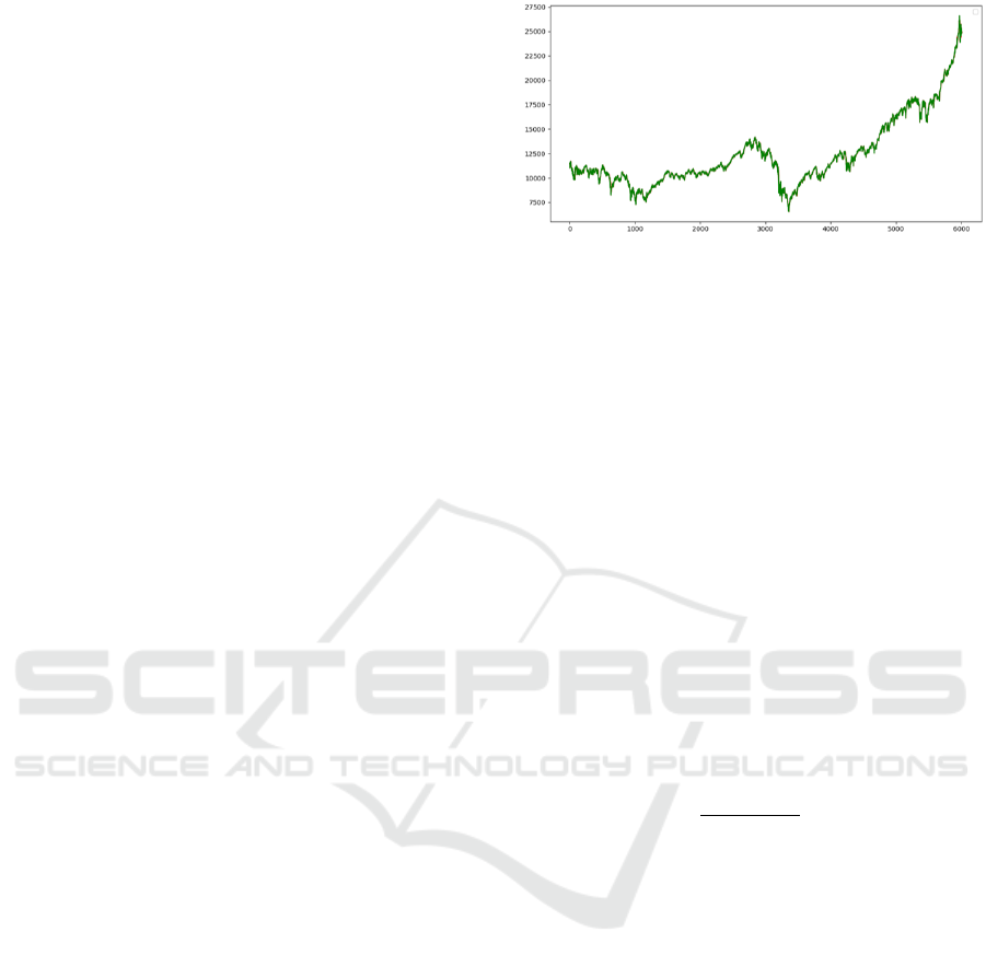
Figure 1: Close price trend of the DJIA between 01/01/2000

and 31/12/2017.

In Figure 1 we can clearly observe that the DJIA

closing values trend is positive on average. To pro-

perly evaluate the models ability in the prediction of

the DJIA prices, we have divided the time series in the

middle, generating a training set between 01/01/2000

and 30/06/2009 (3285 stock prices) and a test set bet-

ween 01/07/2009 and 31/12/2017 (3285 values). The

dimensions of the test set allow to have a high reliabi-

lity with respect to the real predictive capabilities of

the model.

3.2 Data Preparation

In order to compensate for the lack of prices on the

closing days of exchange (holidays, week-ends), we

have executed a ﬁrst step of preprocessing by ap-

plying a convex function , obtaining the new prices

as follow:

+ x

last

(2)

where:

• x

: last price available

• x

last

: ﬁrst price available after the interval of mis-

sing values.

Several works have shown that there is a tempo-

ral lag between the issuance of new public informa-

tion and the decisions taken by the traders. As shown

by the experiments in (Bollen et al., 2011; Domeni-

coni et al., 2017a) the higher correlation between so-

cial mood and the DJIA is obtained by grouping un-

structured data of several days and shifting the pre-

diction for a certain time lag. Similarly, (LeBaron

et al., 1999) illustrated how the new information, pu-

blicly available, can be used within a short time win-

dow to anticipate the market.

According with these approaches, we have aggre-

gated several days of information in order to predict

the closing price of the last day in the list. To do that

we introduced an aggregation (agg) parameter that

identiﬁes the number of days to aggregate, so agg = 3

Dow Jones Trading with Deep Learning: The Unreasonable Effectiveness of Recurrent Neural Networks

145

Figure 2: Example of the DJIA prediction process.

means the data aggregation from the three days, prior

to the prediction day.

The diagram in Figure 2 summarises the DJIA

prediction process. A normalisation process was

applied, both at the opening and the closing pri-

ces, through z-score considering only the information

available at time t.

Z =

X − µ

(3)

For example, the z-score (both for opening and clo-

sing price) on 12/06/2009 was calculated considering

only the prices available until 11/06/2009, leaving out

those starting from 13/06/2009, respecting the con-

ceptual integrity.

3.3 Recurrent Neural Networks

Overview

Recurrent neural networks (RNN) have shown bet-

ter learning capabilities than the traditional FF ones

whenever the data exhibit complex temporal depen-

dencies, which are typical of sequence learning, such

as speech recognition, language modelling and time

series.

As depicted in Figure 3 this is achieved by pro-

viding a retroactive feedback which feed the network

activations from a previous time step as inputs to the

network in order to inﬂuence predictions at the cur-

rent time step. These activations contribute to create

the internal state of the network which can hold long-

term temporal information. This mechanism allows

RNNs to dinamically and autonomously exploit dif-

ferent time windows over the input sequence history

unlike FF networks that are bound to a pre-deﬁned

ﬁxed size window.

While typical FF networks operate as a combina-

torial system, associating an output patterns to an in-

put patterns, RNN networks act as a sequential system

associating an output pattern to an input pattern with

a dependence on an internal state that evolves over

time. The two most popular RNNs are Long Short-

Term Memory (LSTM) (Hochreiter and Schmidhu-

ber, 1997; Gers et al., 1999; Graves, 2013) and Gated

Recurrent Unit (GRU) (Cho et al., 2014).

Both solutions are based on the RNNs but im-

prove them by overcoming some architectural limi-

tations such as the vanishing and exploding gradient

problems which are caused by the weight matrix and

the activation function (or rather its derivative).

In the recurrent networks, the backpropagation of

the error occurs not only for all the levels as well as

in the vanilla backropropagation, typically used in FF

networks, but also for all the time instants provided

as input to the network. This process is called back-

propagation through time (BPTT) and can be summa-

rized as:

∂E

∂W

∑

∂E

∂W

∑

k=0

∂E

∂h

∂c

∂W

(4)

The vanishing/explosion gradient is generated when

the sizes of the time window considered by the net-

work are high. The equation 4 summarizes the pro-

cess by which the error is transported from the current

time t up to the ﬁrst. The crucial point of BPTT is:

∂c

which allows to transport the error from a temporal

instant to the previous one. The vanishing/exploding

gradient problem is raised when the time windows is

wide:

∂c

∏

k<i<=t

∂c

i−1

where the right side of the equation is the product of

the terms of jacobi, therefore:

∏

k<i<=t

∂c

i−1

∏

k<i<=t

diag( f

i−1

))

where f

is the derivative of the activation function.

if k is a small value and t is a big value the re-

sult of the product will be a very large or very small

DATA 2018 - 7th International Conference on Data Science, Technology and Applications

146

Figure 3: Back-propagation through time.

1. U,V,W: are the matrices of the weights shared

among all the temporal instants.

2. E

, E

, . . . E

: are the errors committed in the vari-

ous temporal instants.

3. h

, h

, . . . h

: are the predictions of the network in

the various temporal instants.

4. c

, c

, . . . c

: are the hidden states of the network

in the various temporal instants. They represent

the ’memory’ of the network.

value depending on whether the gradient is > 1 (the

gradient will tend to 0) or < 1 (the gradient will tend

to ∞).

To address this problem, the LSTM networks

have special blocks called memory units in the recur-

rent hidden layer and they use the identity function

(whose derivative is 1) as activation function so as to

keep the error constant during the back propagation

(CEC=Control error carousel).

In order to allow the network to learn, a gate con-

cept has been introduced, which is a unit able to open

or close access to the CEC:

• Input: it allows to add / update information to the

memory cell state C

with respect to the past state.

represent a proposal for the information to

be written within the cell state.

2. i

modulates the proposal (

) of the informa-

tion to be written, or how much ”part of infor-

mation of the proposal to accept”.

The input gate is therefore determined by ’how

much information to forget’ from the cell state at

the previous time (C

t−1

) and ’how much informa-

tion to add’ at the current time (x

• Output: it controls the output ﬂow of cell activa-

tions into the rest of the network and it is determi-

ned by the cell state C

• Forget: In the original proposal (Hochreiter and

Schmidhuber, 1997) the forget gate was not pre-

Figure 4: Architecture of a Long-Short Term Memory Unit.

sent but was added later (Gers et al., 1999) to

prevent LSTM from processing continuous input

streams that are not segmented into subsequences.

The forget gate’s task determines how much infor-

mation of the internal memory unit state should

forget (h

t−1

) and how much information should

add as input at, current time, via the self-recurrent

connection (x

The main difference between LSTM and GRU is

the lack of the memory gates in the GRU networks.

This simpliﬁcation makes GRU faster to train and ge-

nerally more effective than LSTM on smaller training

dataset. On the other hand, the complexity of LSTM

architecture makes them able to correlate longer trai-

ning sequences than the GRU networks.

3.4 Design & Settings of Our Recurrent

Neural Network

We have deﬁned a recurrent neural network architec-

ture based on LSTM with two hidden layers. The pe-

culiarity of this choice is to have in ﬁrst hidden layer

twice the number of neurons contained in than the se-

cond one. This choice derives from the desire to allow

the network to abstract from the speciﬁc information

of the instances, enabling it to identify generic pat-

terns.

The ﬁrst two recurrent hidden layers were trai-

ned using the hyperbolic tangent (tanh) as activation

function while in the output level a linear function was

used. The network was fed using the opening prices

of n days, including the opening price of the target

day, in order to predict the closing price of the target

day by regression. This predicted value has been used

to determine the type of action to be performed as:

action =

(

buy if open − close

predicted

> 0

sell otherwise

(5)

As ﬁrst step, the closing values predicted by the

network using the regression, was used to determine

Dow Jones Trading with Deep Learning: The Unreasonable Effectiveness of Recurrent Neural Networks

147

which action to take. Then the accuracy was calcula-

ted assuming a +1 for each action / class expected

correctly and -1 otherwise. The resulting accuracy

was calculated as:

Accuracy =

correct predictions

total predictions

(6)

The tests were conducted analysing three types of

networks:

1. small network:

• 1 hidden layer: 32 neurons

• 2 hidden layer: 16 neurons

2. medium network:

• 1 hidden layer: 128 neurons

• 2 hidden layer: 64 neurons

3. large network:

• 1 hidden layer: 512 neurons

• 2 hidden layer: 256 neurons

Then three types of gradient optimisation algorithms

have been experimented:

• Momentum: it’s a gradient optimization algo-

rithm whose basic idea is the same as the kine-

tic energy accumulated by a ball pushed down a

hill. If the ball follows the steeper direction, it

will quickly accumulate kinetic energy and when

it meets resistance, it will lose it. Since the gra-

dient of a function indicates the direction along

which it is growing faster, the momentum grows

according to the directions of the past gradients.

If the gradients calculated in the previous steps all

have the same direction, the momentum tends to

grow. If the gradients instead have different di-

rections, the momentum tends to decrease. As

a consequence we will have a faster convergence

than classic Stochastic Gradient Descent limiting

its variability. Weights update happens as

w = w − v

= γv

t−1

+ λ

∂C

∂W

where:

– γ (0.9): is the momentum’s factor

– λ (0.01): is the learning rate

– Decay: 0.0

• Adagrad: address the slow convergence problem

of Stochastic Gradient Descent using an adaptive

learning rate which allows a ﬁne update for fre-

quent parameters and a large update for rare ones.

t+1

(i) = w

(i) −

(i, i) + ε

∂C

∂W

where:

– G

∈ R

dxd

: is a diagonal matrix where every

component on the diagonal (i, i) is the sum of

squared of the gradients from instant 0 to t

– ε: 1e

−7

– λ (0.01): is the learning rate

– Decay: 0.0

• Rmsprop: it is an extension of Adagrad that tries

to solve the problem of the learning rate that tends

to 0 by accumulating the squares of the past re-

stricted gradients within a window w. However,

instead of storing all squared gradients of the last

w instants (which would be inefﬁcient), it uses the

average of the squared gradients at the instant t.

where:

– Learning rate: 0.001

– ρ: 0.9

– ε: 1

−7

– Decay: 0.0

Finally, in order to conduct an analysis of the real

performance of the network architecture a test was

conducted so as to identify the economic gain in terms

of dow points. Each test was conducted by aggrega-

ting the opening prices of several days before the tar-

get date, as described in 3.2, with the goal to predict

the closing price of last day in the aggregate list. The

results were then compared to those obtained by rand-

omly extracting each action between buy and sell.

Testing was performed according to the following

scheme starting from equation 5:

• Only one action can be possessed at a given time.

If the network have chosen to buy and does not

have any previous stock then buy

– The purchase cost is deducted from the capital

– The difference between the opening and closing

price is added to the capital

• If the network has chosen to buy but has already

bought a stock, then keep the stock

– The difference between the opening and closing

price is added to the capital

• If the network has chosen to sell and owns a stock

then sell.

– The opening price is added to the capital

• Otherwise no action is taken

Where capital is equal to 50000 dow points and

represents the amount of money initially available to

the recurrent neural network. The resulting economic

gain is then calculated as:

Gain =

f inal capital

initial capital

(7)

The transaction costs are considered later.

DATA 2018 - 7th International Conference on Data Science, Technology and Applications

148

4 EXPERIMENT SETTINGS AND

RESULTS

4.1 Results with a Positive Trend Time

Series

The table 1 illustrates the average accuracies, achie-

ved by the architecture depicted in Figure 4, obtained

on 6 different runs for each test. These accuracies cor-

respond to 81 different learning models trained accor-

ding to the combination of the number of input days,

of the types of mentioned above network, of the num-

ber of epochs and the kind of the algorithm optimisa-

tion. It is possible to infer from the table that small

and medium networks do not perform as well as the

big ones and that the algorithms adagrad and momen-

tum are more suitable for the type of task considered.

Furthermore 2 input days on average perform better

than a 5 and 10 days.

The hardware conﬁguration on which the solu-

tion have been implemented and experimented con-

sists of 1 GPU NVIDIA Titan Xp 12 GB, 16 cores

Xeon E5-2609 CPU and 32 GB RAM. The work-

station is equipped with Ubuntu 16.04.4 LTS, Py-

thon 3.5.2, keras 2.1.5, tensorﬂow 1.6.0 and NVIDIA

CUDA 9.0.176. With this conﬁguration, each lear-

ning model took on average about 25 minutes to com-

plete the training phase and about 1 minute to com-

plete the testing phase. The training phase has regar-

ded the period between 01/01/2000 and 30/06/2009

and the test phase has occurred in the period between

01/07/2009 and 31/12/2017, where each phase con-

tains 3285 time instant values.

The results of the economic gain achieved by the

learning model with the accuracy of 83%* - which

corresponds in Table 1 to the bold value in the row 2

days and column Momentum 200 epochs - are shown

in Figure 5, where the x axis represents the gain with

respect the initial capital and the y axis the number

of days of input data supplied to the neural network

before the current day in which predicting the clo-

sing price. To proﬁtably increase the gain, the neural

network was also lawfully trained during the testing

phase using only the opening and closing prices prior

to the prediction day.

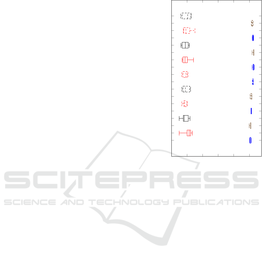
The boxplot in Figure 5 reports the normalized

gain:

(

pro f it, gain > 1.

loss, gain < 1.

Unit gain is the discriminating value that determines

whether the model is able to create proﬁt.

From Figure 5 it is possible to notice how, in the

case of predictions based on random choice, the me-

1 2 3 4

2 days

2 days random

3 days

3 days random

4 days

4 days random

5 days

5 days random

6 days

6 days random

7 days

7 days random

8 days

8 days random

9 days

9 days random

10 days

10 days random

Figure 5: Economic gains, in terms of dow points, calcula-

ted according to the equation 7 according to the test between

01/01/2000 and 31/12/2017 with 200 training epochs, with

optimisation algorithm Momentum and with the neural net-

work composed by 512 and 256 neurons in the level 1 and

2 respectively, see Table 1.

dian is below the unit value most of the time. This in-

dicates that random prediction always leads to a loss.

On the contrary, basing the choice using model 4 le-

ads to a gain that is 5.09 times the initial capital.

In this last case, it is evident how the variability

is considerably lower than the random based appro-

ach. Obviously the difference between percentile 25

and percentile 75 is much inferior than the same diffe-

rence when the actions to be performed are randomly

chosen. This leads us to conclude that the forecast is

much more stable and reliable if carried out with the

illustrated model.

The gain obtained by our LSTM learning model

with the accuracy of 83% (highlighted with an aste-

risk in Table 1), has outperformed the gains achieved

with neural networks applied to DJIA (O’Connor and

Madden, 2006). The authors in (O’Connor and Mad-

den, 2006) have applied a FF model to a test set in-

terval between the years 1987 and 2002, obtaining a

maximum ROI (Return of Investment) of 23.42% per

year, excluding transaction fees. The data inputs their

provided to the model are the opening price of the

dow jones and other external indicators, including the

Dow Jones Trading with Deep Learning: The Unreasonable Effectiveness of Recurrent Neural Networks

149

Table 1: Accuracies of the implemented neural network architecture, whose unit is depicted in Figure 4, in response to changes

in the number of input days, training epochs, network sizes and types of optimisation algorithms. The learning model we used

in the trading experiments is the one corresponding to 83%*.

Test set accuracies between 01/07/2009 and 31/12/2017

Adagrad Momentum Rmsprop

Epochs 50 100 200 50 100 200 50 100 200

2 days s: 39% s: 40% s:64% s: 69% s: 71% s: 72% s: 72% s: 68% s: 70%

m: 41% m: 81% m: 79% m: 78% m: 74% m: 80% m: 71% m: 61% m: 69%

l: 84% l: 80% l: 47% l: 70% l: 70% l: 83%* l: 68% l: 79% l: 70%

5 days s: 52% s: 79% s: 66% s: 68% s: 68% s: 71% s: 55% s: 51% s: 68%

m: 74% m: 59% m: 71% m: 68% m: 74% m: 78% m: 73% m: 70% m: 68%

l: 69% l: 80% l: 79% l: 71% l: 74% l: 83% l: 67% l: 68% l: 66%

10 days s: 68% s: 68% s: 65% s: 69% s: 73% s: 71% s: 68% s: 64% s: 66%

m: 70% m: 78% m: 54% m: 71% m: 73% m: 74% m: 68% m: 68% m: 68%

l: 80% l: 86% l: 45% l: 80% l: 79% l: 75% l: 68% l: 79% l: 64%

s: 32 neurons in level 1, 16 in level 2

m: 128 neurons in level 1, 64 in level 2

l: 512 neurons in level 1, 256 in level 2

opening price of the previous 5 days, the 5-day gra-

dient and the USD/YEN, USD/GBP, USD/CAN con-

version rates. Our LSTM-based model has achieved

on average a ROI of 56.5% per year, which produces

a cumulative proﬁt of 254,000 dow points from an ini-

tial capital of 50000 dow points, that is more than 5

times the initial capital, which is also larger than the

18.48 ROI achieved with the same LSTM technology

in (Bao et al., 2017).

Table 2 compares the performances obtained with

our selected LSTM-based model and the one based on

FF networks considering the same test procedure used

in 1. The results show that LSTM networks achieve a

higher accuracy which is then translated into a greater

cumulative proﬁt.

Table 2: Performance, obtained on 6 runs, comparison bet-

ween the LSTM based model and the one based on FF net-

works with agg = 2, with 200 epochs of training and Mo-

mentum as gradient optimisation algorithm, with (S)mall,

(M)edium and (L)arge networks’ sizes.

Test set accuracies comparison

Feed-Forward LSTM

S M L S M L

63% 65% 68% 72% 80% 83%

Cumulative Proﬁts (times initial capital)

Feed-Forward LSTM

S M L S M L

3.47 3.59 3.56 4.03 4.33 5.09

The graph (C) of Figure 6 compares the closing

prices predicted by the model, trained for 200 epochs

with agg = 2 and Momentum as gradient optimisa-

tion algorithm, with real prices. The average error

committed, by regression, by the model, in the en-

tire period, is 113.09 dow points and the relative σ is

157.92 dow point where σ of close prices in test set

is 4140.74. This denotes the high capacity of deep

networks (in particular LSTM) to extract meaningful

information from a noisy context.

The great ability to forecast closing prices transla-

tes into a good ability to determine the action to be ta-

ken, according with equation 5, in order to maximize

the economic return. The graph (A) of ﬁgure 6 illus-

trates the cumulative proﬁt trend during the test pe-

riod between 01/07/2009 and 31/12/2017 both gross

and net of fees considering 2 days of aggregation,

200 epochs of training and Momentum as optimiza-

tion algorithm. In the latter case we have assumed a

ﬁxed commission of 15‰ obtaining 251336.21 dow

points or 1.35% less than the case without commissi-

ons which is 254786.55.

The graph (B) of Figure shows the trend of daily

proﬁt with the inverted DJIA time series, which, as

reported in the graph (D), has a negative trend on

average. In the latter case, the proﬁt derives from the

daily volatility of the stock prices. It is also interes-

ting to highlight, as in correspondence with the grea-

ter drop in the value of the stock prices, the network

has decided to ’keep’ the stocks (not buy and not sell).

Here the network has extracted some form of pattern

that led it to decide to minimize losses by assuming a

neutral attitude.

Labelling as False positive and False negative re-

spectively the actions in which the network bought

and sold erroneously, the calculated f1 measure is

0.82 supporting the hypothesis that the model is able

to catch patters in the data and with which performing

reliable predictions.

Finally, the minimum capital needed was calcu-

lated so that the capital would never be negative du-

DATA 2018 - 7th International Conference on Data Science, Technology and Applications

150

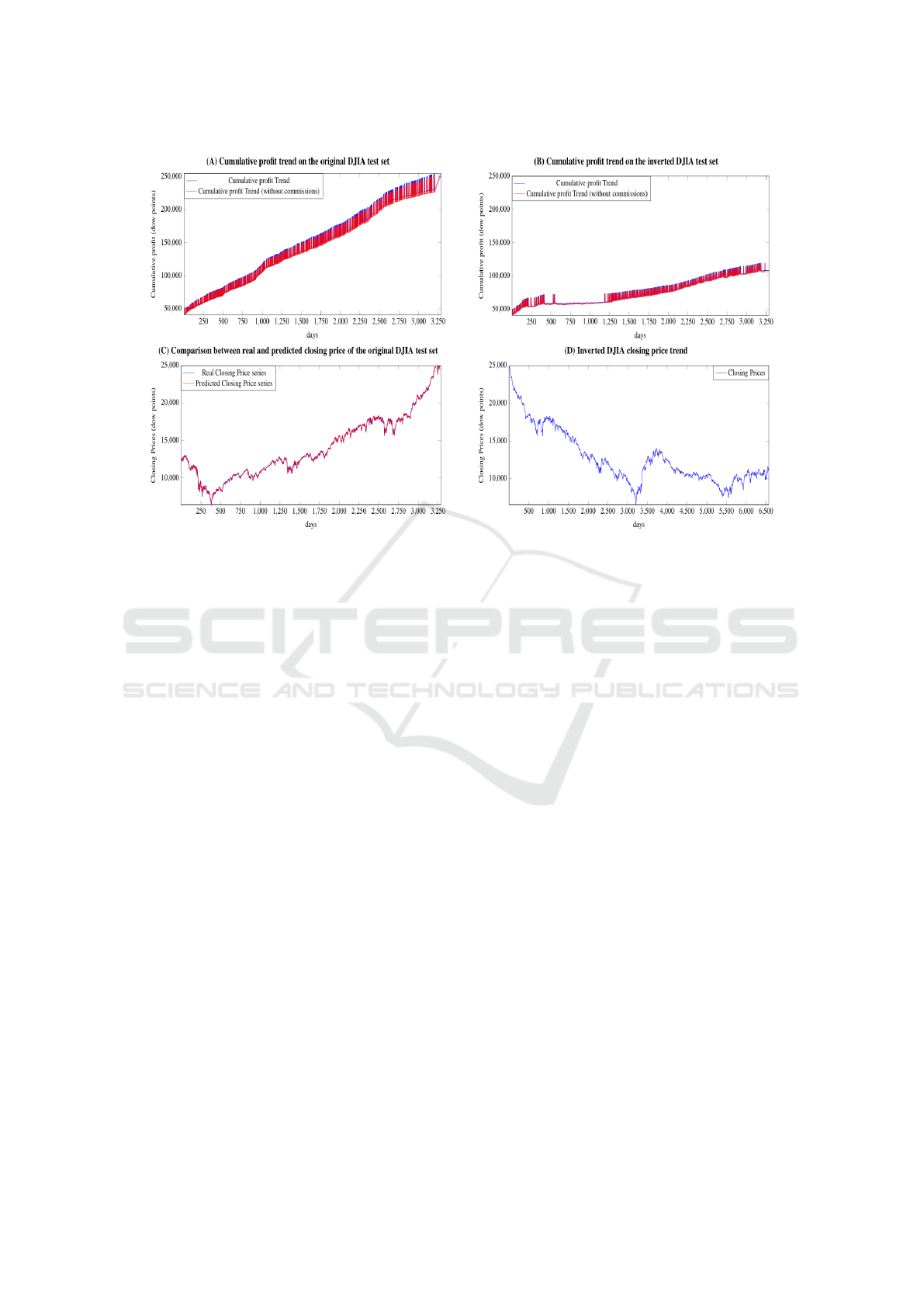
Figure 6: (A) Daily proﬁt trend with and without commissions (ﬁxed at 15 ‰) for the DJIA between the 01/07/2009 and

31/12/2017 with an initial capital of 50000 dow points

(B) Daily proﬁt trend with and without commissions (ﬁxed at 15 ‰) for the inverted DJIA time series between the 30/06/2009

and 01/01/2000 with an initial capital of 50000 dow points; the training phase is between 31/12/2017 and 01/07/2009

(C) Comparison between real and predicted closing price as reported in Table 1 for the DJIA with agg = 2, with 200 epochs

of training and Momentum as gradient optimisation algorithm.

(D) Close price trend of the inverted DJIA time series between the 31/12/2017 and 01/01/2000.

ring the entire forecast period. Of all the experiments

conducted, the minimum capital required in the worst

case was 11878.28 dow points.

4.2 Results with a Negative Trend Time

Series

The previous section illustrated the results of our

RNN achieved on the DJIA time series between the

year 2000 and the year 2017. Observing the time se-

ries it is possible to notice that its trend is on average

positive, which might concealing the real predictive

capabilities of the model.

To obtain a counter-test of the results obtained in

4.1, we have tested the same learning model used in

the previous subsection, on the same but inverted time

series, that is a negative trend on average, where the

ﬁrst day of the series is the 31/12/2017 and the last

day is the 01/01/2000.

Then we have reran the most signiﬁcant tests con-

sidering also the random counterparts. In particular,

the tests were conducted on the large network with

512 neurons in the ﬁrst hidden layer and 256 in the se-

cond hidden layer, moreover it has been trained with

200 epochs from the aggregation of the opening pri-

ces of 7 and 8 days prior to the target day. The test

policies are the same deﬁned in 4.1 and the ﬁnal gain

is computed according to the equation 7. The gains

achieved, prior to commission fees, are the following:

with 7 days is 2.23 versus 0.74 of the random appro-

ach, which corresponds to a loss of 26%, and with

8 days is 2.12 against 0.75 of the random approach,

which amount to a loss of 25%.

This experiment shows that the gain is halved

compared to that obtained with the original DJIA his-

torical series, but it still leads to a proﬁt of more than

twice the initial capital with both cases of 7 and 8

days. The gain obtained through a model operating

random choices is about 25% lower than that obtained

on the original DJIA time series, however, leading to

losing part of the initial capital.

This last test is particularly relevant as it clearly

shows how the proposed solution obtains signiﬁcant

gains even in the presence of a time series with a

negative averagely trend. Moreover from the graph

(B) of Figure 6, we can see that the selected lear-

ning model almost never performs trading actions in

test interval between the day number 600 and 1200,

which corresponds in the graph (D) to the interval be-

tween the day number 3885 (i.e. 3285+600) and 4485

Dow Jones Trading with Deep Learning: The Unreasonable Effectiveness of Recurrent Neural Networks

151

(3285+1200), that is a long consecutive test period of

decreasing of the inverted DJIA. This highlights that

the solution has also learned when it is better to re-

frain from trading.

5 CONCLUSION

In this work, we have analysed the predictive capa-

bilities on the DJIA index of a simple solution based

on novel deep recurrent neural networks, which in se-

veral research areas have shown superior capabilities

of detecting long term dependencies in sequences of

data, such as in speech recognition and in text under-

standing. The aim of our work was to move away

from the latest complex trends, in terms of stock mar-

ket prediction based on the use of non-structured data

(tweets, ﬁnancial news, etc.), in order to focus more

simply on the stock time series. From this viewpoint

the work follows the philosophy of the ARIMA ap-

proach proposed in 1970 by Box and Jenkins but ex-

perimenting advanced approaches.

Our tests have shown that the proposed solution is

able to obtain a prediction accuracy of about 83% and

a proﬁt of more than 5 times the initial capital, out-

performing the state-of-the-art. The tests have also

shown how the predictions beneﬁt from a lower va-

riability compared to that obtained with an approach

operating random choices.

The work can be extended to a scenario of paral-

lel trading with multiple stocks, also investigating and

exploiting possible correlations among different mar-

ket indexes. Another possible improvement is to pre-

dict the best trading action according to forecasts of

stock price movements referred to two or more days

in the future. This strategy may lead to the identiﬁca-

tion of additional recurring patterns able to exploit the

time lag in the reactivity of stock market as supposed

in (LeBaron et al., 1999).

REFERENCES

Abe, M. and Nakayama, H. (2018). Deep learning for fore-

casting stock returns in the cross-section. arXiv pre-

print arXiv:1801.01777.

Akita, R., Yoshihara, A., Matsubara, T., and Uehara, K.

(2016). Deep learning for stock prediction using nu-

merical and textual information. In Computer and In-

formation Science (ICIS), 2016 IEEE/ACIS 15th In-

ternational Conference on, pages 1–6. IEEE.

Atsalakis, G. S. and Valavanis, K. P. (2009a). Forecasting

stock market short-term trends using a neuro-fuzzy

based methodology. Expert systems with Applicati-

ons, 36(7):10696–10707.

Atsalakis, G. S. and Valavanis, K. P. (2009b). Surveying

stock market forecasting techniques–part ii: Soft com-

puting methods. Expert Systems with Applications,

36(3):5932–5941.

Bao, W., Yue, J., and Rao, Y. (2017). A deep learning

framework for ﬁnancial time series using stacked au-

toencoders and long-short term memory. PLOS ONE,

12(7):1–24.

Bollen, J., Mao, H., and Zeng, X. (2011). Twitter mood

predicts the stock market. Journal of computational

science, 2(1):1–8.

Box, G. E. P. and Jenkins, G. (1970). Time Series Analy-

sis, Forecasting and Control. Holden-Day, Inc., San

Francisco, CA, USA.

Cao, Q., Leggio, K. B., and Schniederjans, M. J. (2005).

A comparison between fama and french’s model and

artiﬁcial neural networks in predicting the chinese

stock market. Computers & Operations Research,

32(10):2499–2512.

Cho, K., van Merri

enboer, B., G

ulc¸ehre, C¸ ., Bahdanau, D.,

Bougares, F., Schwenk, H., and Bengio, Y. (2014).

Learning phrase representations using rnn encoder–

decoder for statistical machine translation. In Pro-

ceedings of the 2014 Conference on Empirical Met-

hods in Natural Language Processing (EMNLP), pa-

ges 1724–1734, Doha, Qatar. Association for Compu-

tational Linguistics.

di Lena, P., Domeniconi, G., Margara, L., and Moro, G.

(2015). GOTA: GO term annotation of biomedical li-

terature. BMC Bioinformatics, 16:346:1–346:13.

Ding, X., Zhang, Y., Liu, T., and Duan, J. (2015). Deep

learning for event-driven stock prediction. In Ijcai,

pages 2327–2333.

Domeniconi, G., Masseroli, M., Moro, G., and Pinoli, P.

(2016). Cross-organism learning method to discover

new gene functionalities. Computer Methods and Pro-

grams in Biomedicine, 126:20–34.

Domeniconi, G., Moro, G., Pagliarani, A., and Pasolini, R.

(2017a). Learning to predict the stock market dow

jones index detecting and mining relevant tweets.

Domeniconi, G., Moro, G., Pagliarani, A., and Pasolini, R.

(2017b). On deep learning in cross-domain sentiment

classiﬁcation. In Proceedings of the 9th Internatio-

nal Joint Conference on Knowledge Discovery, Know-

ledge Engineering and Knowledge Management - (Vo-

lume 1), Funchal, Madeira, Portugal, November 1-3,

2017., pages 50–60.

Esteva, A., Kuprel, B., Novoa, R. A., Ko, J., Swetter, S. M.,

Blau, H. M., and Thrun, S. (2017). Dermatologist-

level classiﬁcation of skin cancer with deep neural net-

works. Nature, 542(7639):115–118.

Fama, E. F. (1970). Efﬁcient capital markets: A review of

theory and empirical work. The journal of Finance,

25(2):383–417.

Fischer, T. and Krauss, C. (2017). Deep learning with long

short-term memory networks for ﬁnancial market pre-

dictions. European Journal of Operational Research.

Fisher, I. E., Garnsey, M. R., and Hughes, M. E. (2016). Na-

tural language processing in accounting, auditing and

ﬁnance: A synthesis of the literature with a roadmap

DATA 2018 - 7th International Conference on Data Science, Technology and Applications

152

for future research. Intelligent Systems in Accounting,

Finance and Management, 23(3):157–214.

Gers, F. A., Schmidhuber, J., and Cummins, F. (1999). Lear-

ning to forget: Continual prediction with lstm. Neural

Computation, 12:2451–2471.

Gidofalvi, G. and Elkan, C. (2001). Using news articles to

predict stock price movements. Department of Com-

puter Science and Engineering, University of Califor-

nia, San Diego.

Graves, A. (2013). Generating sequences with recurrent

neural networks. arXiv preprint arXiv:1308.0850.

Hochreiter, S. and Schmidhuber, J. (1997). Long short-term

memory. Neural computation, 9(8):1735–1780.

Khashei, M., Bijari, M., and Ardali, G. A. R. (2009). Impro-

vement of auto-regressive integrated moving average

models using fuzzy logic and artiﬁcial neural net-

works (anns). Neurocomputing, 72(4-6):956–967.

Khashei, M., Bijari, M., and Ardali, G. A. R. (2012). Hybri-

dization of autoregressive integrated moving average

(arima) with probabilistic neural networks (pnns).

Computers & Industrial Engineering, 63(1):37–45.

Krizhevsky, A., Sutskever, I., and Hinton, G. E. (2012).

Imagenet classiﬁcation with deep convolutional neu-

ral networks. In Proceedings of the 25th Internatio-

nal Conference on Neural Information Processing Sy-

stems - Volume 1, NIPS’12, pages 1097–1105, USA.

Curran Associates Inc.

LeBaron, B., Arthur, W. B., and Palmer, R. (1999). Time

series properties of an artiﬁcial stock market. Journal

of Economic Dynamics and control, 23(9-10):1487–

1516.

Lee, C.-M. and Ko, C.-N. (2011). Short-term load forecas-

ting using lifting scheme and arima models. Expert

Systems with Applications, 38(5):5902–5911.

Lee, K., Yoo, S., and Jongdae Jin, J. (2007). Neural network

model vs. sarima model in forecasting korean stock

price index (kospi). 8.

Lin, M.-C., Lee, A. J., Kao, R.-T., and Chen, K.-T. (2011).

Stock price movement prediction using representative

prototypes of ﬁnancial reports. ACM Transactions on

Management Information Systems (TMIS), 2(3):19.

Lo, A. W. and MacKinlay, A. C. (1988). Stock market pri-

ces do not follow random walks: Evidence from a sim-

ple speciﬁcation test. The Review of Financial Studies,

1(1):41–66.

Lo, A. W. and Repin, D. V. (2002). The psychophysiology

of real-time ﬁnancial risk processing. Journal of cog-

nitive neuroscience, 14(3):323–339.

Malkiel, B. G. (1973). A Random Walk Down Wall Street.

Norton, New York.

Malkiel, B. G. (2003). The efﬁcient market hypothesis

and its critics. Journal of economic perspectives,

17(1):59–82.

Merh, N., Saxena, V. P., and Pardasani, K. R. (2010). A

comparison between hybrid approaches of ann and

arima for indian stock trend forecasting. Business In-

telligence Journal, 3(2):23–43.

Mitra, S. K. (2009). Optimal combination of trading rules

using neural networks. International business rese-

arch, 2(1):86.

Mostafa, M. M. (2010). Forecasting stock exchange mo-

vements using neural networks: Empirical evidence

from kuwait. Expert Systems with Applications,

37(9):6302–6309.

O’Connor, N. and Madden, M. G. (2006). A neural

network approach to predicting stock exchange mo-

vements using external factors. Knowl.-Based Syst.,

19(5):371–378.

Olson, D. and Mossman, C. (2003). Neural network fore-

casts of canadian stock returns using accounting ra-

tios. International Journal of Forecasting, 19(3):453–

465.

Schumaker, R. and Chen, H. (2006). Textual analysis of

stock market prediction using ﬁnancial news articles.

AMCIS 2006 Proceedings, page 185.

Schumaker, R. P. and Chen, H. (2009). Textual analysis

of stock market prediction using breaking ﬁnancial

news: The azﬁn text system. ACM Transactions on

Information Systems (TOIS), 27(2):12.

Soni, S. (2011). Applications of anns in stock market pre-

diction: a survey. International Journal of Computer

Science & Engineering Technology, 2(3):71–83.

Sterba, J. and Hilovska, K. (2010). The implementation of

hybrid arima neural network prediction model for ag-

gregate water consumption prediction. AplimatJour-

nal of Applied Mathematics, 3(3):123–131.

Tetlock, P. C. (2007). Giving content to investor sentiment:

The role of media in the stock market. The Journal of

ﬁnance, 62(3):1139–1168.

Wang, W., Li, Y., Huang, Y., Liu, H., and Zhang, T. (2017).

A method for identifying the mood states of social net-

work users based on cyber psychometrics. Future In-

ternet, 9(2):22.

Wikipedia contributors (2018). Financial statement — Wi-

kipedia, the free encyclopedia. [Online; accessed 20-

May-2018].

Yahoo! FinanceYahoo! Finance (2000-2017). Dow jones

industrial average (djia). http://bit.ly/2rozaW8.

Dow Jones Trading with Deep Learning: The Unreasonable Effectiveness of Recurrent Neural Networks

153