ADAPTIVE SMITH PREDICTIVE CONTROL OF NON-LINEAR

SYSTEMS USING NEURO-FUZZY HAMMERSTEIN MODELS

José Vieira

Escola Superior de Tecnologia de Castelo Branco, Departamento de Engenharia Electrotécnica, Av. Empresário, 6000

Castelo Branco, Portugal

Alexandre Mota

Departamento de Electrónica e Telecomunicações, Universidade de Aveiro, 3810 Aveiro, Portugal

Keywords: Adaptive control, Smith predictive control, Hammerstein models, neuro-fuzzy modelling, on-line

identification, recursive least square and covariance matrix

Abstract: This paper proposes an Adaptive Smith Predictor Controller (ASPC) based on Neuro-Fuzzy Hammerstein

Models (NFHM) with on-line non-linear model parameters id

entification. The NFHM approach uses a zero-

order Takagi-Sugeno fuzzy model to approximate the non-linear static function that is tuned off-line using

gradient decent algorithm and to identify the linear dynamic function it is used the Recursive Least Square

estimation with Covariance Matrix Reset (RLSCMR). This algorithm has the capability of follow fast and

slow dynamic parameter changes. The proposed ASPC has special capabilities to control non-linear systems

that have gain, time delay and dynamic changes through time. The implementation of the ASPC is made in

two steps: first, off-line estimation of the non-linear static parameters that will be used to “get linear” the

non-linearity of the system and second, on-line identification of the linear dynamic parameters updating

direct and inverse models used in the ASPC. As an illustrative example, a gas water heater system is

controlled with the ASPC. Finally, the control results are compared with the results obtained with the Smith

Predictive Controller based in a Semi-Physical Model (SPMSPC).

This work was supported in part by the Portuguese Government through the PREDEP program.

1 INTRODUCTION

Industry control processes presents many

challenging problems, including non-linear dynamic

behaviour, uncertain time delay and time varying

parameters. During the last decades, a very

promising model based control solution used in

industry processes with time delay is the

predictive/Smith predictive model based controller.

In this algorithm it is important to choose the right

model representation of the linear/non-linear system.

The model should be accurate and robust for all

working points, with a simple mathematical

representation and with a transparent representation

that makes it interpretable. The most common non-

linear modelling methods are: the NARX and

NAARX models, neural-networks models fuzzy

models and Hammerstein and Wiener models.

When the knowledge of the control systems does not

ist or th

e process is subject to changes in its

dynamic characteristics it is important to use an

adaptive control algorithm.

There are two types of model based controllers: off-

ine t

uned model based controllers (Abonyi el at.,

2000), (Pottmann and Seborg 1997), (Vieira el at.,

2003) and adaptive controllers with on-line

parameters identification as (Abonyi el at., 1999)

and (Fink el at., 2001).

This paper presents a simple adaptive model based

ntro

ller that uses the NFHM approach (Vieira el

at., 2004b) with a modification that gives to the

algorithm the capability of identify on-line the linear

dynamic parameters of the linear part of the global

Vieira J. and Mota A. (2004).

ADAPTIVE SMITH PREDICTIVE CONTROL OF NON-LINEAR SYSTEMS USING NEURO-FUZZY HAMMERSTEIN MODELS.

In Proceedings of the First International Conference on Informatics in Control, Automation and Robotics, pages 62-69

DOI: 10.5220/0001131900620069

 SciTePress

model. Hammerstein model approach gives simple

and interpretable models that facilitate the

identification and its integration on control schemes.

Based on this presupposes, it is proposed a simple

solution for the adaptive control of non-linear

systems that presents uncertain, time delay and time

varying dynamic parameters. In time variant

processes, the non-linear static functions are usually

fixed through time (permitting tuning off line) and

the changes are in its dynamic behaviour so it is

necessary to identify the linear dynamic parameters

on line (Fink el at., 2001).

Section 2 and 3, describes the Neuro-Fuzzy

Hammerstein Model structure and the modified

identification method. For the non-linear static

function approximation it is used a zero-order

Takagi-Sugeno fuzzy model tuned with gradient

decent algorithm. With the inverse of this non-linear

static function the non-linear system will be linear.

For the linear variant dynamic function

approximation it is used the on-line recursive least

square parameter estimation with reset of covariance

matrix algorithm. This algorithm has the capability

of identify fast and slow dynamic parameter

changes.

The challenger for non-linear on-line identification

is to guarantee that all parameters of the varying

dynamic model are correctly identifies even in the

presence of a varying time delay and a noisy system.

Section 4, describes the ASPC that is implemented

in two steps: first, off-line estimation of the non-

linear static parameters and second, on-line

identification of the linear dynamic parameters

updating direct and inverse models of the system

used in the controller.

Section 5, shows the control results using the ASPC

applied in to a domestic gas water heater system.

The results are compared with the ones achieved

with the Smith Predictive Controller based in a

Semi-Physical Model (Vieira el at., 2004a).

Finally, in section 6, the conclusions and future

works are pointed.

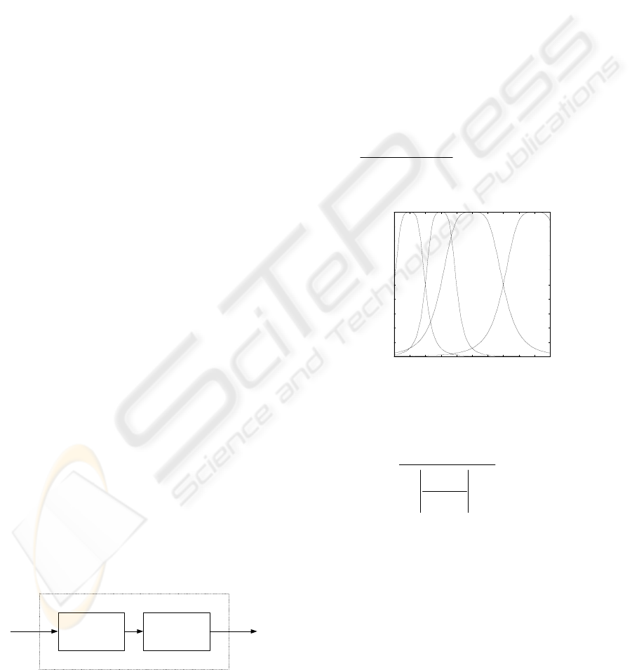
2 STRUCTURES OF THE NFHM

The NFHM consists of a series connection of a non-

linear static function f(.) and a linear dynamic

function G(s) as shown in Figure 1.

Figure 1: Hammerstein Model.

It is proposed, that the non-linear static function

would be approximated by a zero-order Takagi-

Sugeno fuzzy model

The fuzzy model function f(.) can be formulated

as a set of r local constant functions z

, …, z

where d

,…, d

are constant parameters that are

conjugated in the form of rules:

1..r1..r1..r1..r

dz THEN A isu IF:R =

(1)

where A

1..r

are the antecedent fuzzy sets for the input

u and d

1..r

are the consequent constant parameters.

All fuzzy sets are bell shaped type membership

functions see Figure 2.

From a given u, the output of the fuzzy model z is

inferred by computing the weight average of the rule

consequents:

∑

(u)

(2)

Umin

0.5

Umax

...

0.0

1.0

Figure 2: Bell shaped membership functions of the

fuzzy model (1..r fuzzy sets).

where,

bb*2

ccu

(u)A

−

(3)

is the membership function of the input u relative to

the fuzzy set A

and aa

, bb

and cc

are parameters

for adjust the shape and centre of the fuzzy set i.

The number of rules/number of fuzzy sets will

depend only of the complexity of the real static non-

linear function. After define the number of fuzzy

set/rules the non-linear parameters aa

, bb

and cc

for

all fuzzy sets and the linear parameters d

for i=1..r

rules should calculate.

Non-Linear Transfer Function

f(.)

G(s)

yuz

The second part of the structure of the NFHM is

the definition of the linear dynamic function G(s).

ADAPTIVE SMITH PREDICTIVE CONTROL OF NON-LINEAR SYSTEMS USING NEURO-FUZZY

HAMMERSTEIN MODELS

This G(s) function is an n order linear system

represented in discrete domain by equation 4

nu)ndz(k

b...nd)z(k

ny)y(k

a...2)y(k

a1)y(k

ay(k)

−−++−+

−++−+−=

(4)

where a

, a

, …, a

and b

, b

, …, b

are the

numeric parameters of dynamic linear system. nu+1

and ny indicated the order of the regressors need for

each variable and nd is the discrete time delay.

The global mathematical equation of the NFH global

model is illustrated in equation 5.

⎟

⎠

⎞

⎜

⎝

⎛

⎟

⎠

⎞

⎜

⎝

⎛

∑

−

∑

−

∑

−

∑

−

−++−+−=

nu))-nd(u(k

...

nd))(u(k

ny)y(k

a...2)y(k

a1)y(k

ay(k)

(5)

3 IDENTIFICATION OF THE

NFHM

In time variant processes, the non-linear static

functions are usually fixed through time so the

parameters identification could be made off-line.

Otherwise, the linear dynamic functions could

present some changes in its dynamic behaviour so it

is better to identify its parameters on line. For the

identification of the non-linear static function the

used training data should fulfil several requirements.

The control signal u(k) applied to the system should

be a step signal with a large number of steps in its

universe [Umin, …, Umax]. The large number of

steps is very important to get the exact non-linearity

of the system (number of steps depends on the non-

linearity type function). Another important

requirement is the time (number of samples) that the

step control signal should be maintained with out

any changes. This time should be long enough for

the system achieving the stationary state (at least 5

time constants of the system that achieves 99.1% of

the stationary state). The figure 3 illustrates a typical

training control signal u.

With this type of training signal it is possible to

get, first, the stationary state data for training the

non-linear static function, and second, the transitory

data for the initialisation of the dynamic linear

function.

For training the non-linear static function there

was used the two vectors with NS stationary state

samples u

) and y

) obtained as shows figure 3

Time (sec)

uUmax

Umin

...

y(k

)

u(k

)

i=1..NS

Figure 3: Typical training control signal.

(NS);y (2);...;y (1);yy

(NS);u (2);...;u (1);uu

ssssssss

(6)

For the initialisation of the dynamic linear

function it is used all (N) samples of all u (static and

dynamic samples).

y(N); y(2);...; y(1);y

u(N); u(2);...; u(1);u

(7)

The identification method imposes that all gain of

the system is included in the non-linear static

function and the dynamic linear function will have a

unitary gain, at least in the off-line training phase.

The non-linear static function is approximated by

a zero-order Takagi Sugeno fuzzy modelled. The

tuning of the parameters used in the fuzzy model can

be considered as a numerical optimisation

procedure. Among the methods that have been

implemented so far the gradient decent adaptation

method permits accurate learning of all parameters

of the fuzzy modelled. The fuzzy model is

parameterised by the following parameters.

{

}

setsfuzzy rules/nº1..r i ; d ,cc ,bb ,aa

iiii

(8)

The objective is to minimize the global prediction

vector error between the model and the plant

outputs. Therefore, the gradient decent method tends

ICINCO 2004 - SIGNAL PROCESSING, SYSTEMS MODELING AND CONTROL

to decrease the quadratic objective function based on

the vector error

()

1..Nllength of vectorsyy

ssmm

=−=

(9)

with z=y in stationary state, y

is the

approximation output vector of the fuzzy model The

parameter set

Ψ, of the fuzzy model is changed via

the following iterative (j) learning rule:

(j)

e(j)

-(j)(j)(j)1)(j

λψψψ

∂

=∆+=+

(10)

where

λ is the learning rate parameter, which

controls the learning velocity of the algorithm. The

number of iterations will depend on the decreasing

of the total vector error

∑e using the learning

vectors. When the algorithm achieves a predefine

small value or a maximum number of iterations the

iterative algorithm stops.

The partial derivatives of the model error e with

the respect to the parameters of the fuzzy model are

given by:

∑

⎟

⎠

⎞

⎜

⎝

⎛

∂

⎟

⎠

⎞

⎜

⎝

⎛

∂

=∆+=+

l 1

imm

aaiiii

(j)d

(j)y

e(j)

-(j)d

(j)d

e(j)

...

(j)cc

e(j)

...

(j)bb

e(j)

l)(j,aa

l)(j,A

l)(j,R

l)(j,Ry

l)(j,y

l)e(j,

(j)aa

e(j)

(j)aa

e(j)

-(j)aa(j)aa(j)aa1)(jaa

(11)

In the initialisation, the antecedent membership

functions and the consequent constant functions are

equidistantly distributed over the input and output

respective universes of discourse.

The second part of the learning algorithm is the

definition of the linear dynamic function parameters.

The first question that arises is the choice of the

order/significant regressors of the modelled. To find

the significant regressors of the system it could be

used à priori knowledge of the system or the polo-

zero cancellation method.

To estimate the initial a=a

, a

, …, a

and b=b

, b

, …, b

vectors, it was used the Least Square

algorithm.

The modification of the NFHM approach is exactly

here in the identification of the linear dynamic

parameters. In this method this parameters are

calculated on-line with recursive least square

algorithm with reset of covariance matrix

(RLSCMR) as expressed in equation 12,

[

]

[]

[

]

()

nu0ny1

1)P(k (k) UK(k)I

P(k)

U(k)1)P(k (k)U-

U(k)1)P(k

K(k)

1)ab(k (k)Uy(k)(k)

(k) K(k)1)ab(kab(k)

nu)-td-z(k ... td)-z(k

ny)-y(k ... 1)-y(k U(k)

(k)...b (k)b (k)a ... (k)a ab(k)

u(k) f z(k)

−−

−

−−=

+−=

(12)

where ab(k) is the vector with the instant k estimated

parameters,

is the learning rate and P(k) is the

covariance matrix. The Reset Covariance Matrix

(RCM) algorithm is used for a fast convergence in

the identified parameters. If the error

ε(k) is bigger

than a pre-defined value the covariance matrix P is

reset (starting values).

4 ADAPTIVE SMITH PREDICTOR

CONTROL STRUCTURE

The Adaptive Smith Predictive Controller is based in

the Internal Model Controller (IMC) architecture

and is implemented in two phases. First is the off-

line estimation of the non-linear static parameters.

Second is the on-line identification of the linear

dynamic parameters updating the direct and inverse

models of the system, as illustrated in figure 4. Off-

line, with the inversion of the non-linear static

function, it is possible to transform the non-linear

plant in to an approximate “linear” plant. Finally in

closed loop control, iteration-by-iteration, the linear

dynamic parameters are recalculated and updated.

ADAPTIVE SMITH PREDICTIVE CONTROL OF NON-LINEAR SYSTEMS USING NEURO-FUZZY

HAMMERSTEIN MODELS

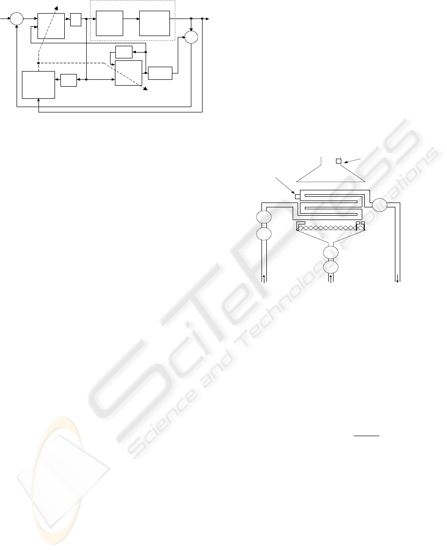
Figure 4: ASPC constituent blocks.

The ASPC separates the time-delay of the plant

from the model of the plant, so it is possible to

predict the y(k)

n steps earlier (n= digital time-

delay), compensating the negative time-delay effects

in the control results. The incorrect prediction of the

time delay may lead to aggressive control if the

time-delay is under estimated or conservative

control if the time-delay is over estimated (Tan

at.

, 2002).

5 ILLUSTRATIVE EXAMPLE:

GAS WATER HEATER

TEMPERATURE CONTROL

The global system has three main blocks: the gas

water heater, a micro-controller board and a personal

computer. The micro-controller board has three

modules, all controlled by the flash-type micro-

controller PHILIPS 89C51RD. The Sensors and

Actuators module is used to read and actuate the

inputs and outputs of the system. The Security

module that is used for the supervision and control

of the security conditions. The Communication

module that is used for the acquisition/monitoring of

the system data to the personal computer.

After a small description of the global system, it

will be made a small description of the gas water

heater system and its characteristics, for a detailed

description see (Vieira

el at. 2003) and it ends with

the definition, identification and comparison of the

proposed ASPC with the SPMSPC (Vieira

el at.

2004a).

5.1 System Description

The gas water heater is a multiple input single output

(MISO) system. The objective is to control the

output water temperature, called hot water

temperature (hwt). This variable depends of the cold

water temperature (cwt), water flow (wf), gas flow

(gf) (applied power) and the gas water heater

dynamics. Considering that the cold water

temperature is almost constant, the final objective is

to control the delta water temperature (

∆t)

(difference between hot and cold water

temperatures) reducing the number of inputs.

Plant

r(k)

-1

y(k)z(k)

-1

(.)

u(k)

G(z)

-1

(z)

"Linearisation" of the plant

e(k)

RLS

with

RCM

-td (k)

The gas water heater is physically composed by a

gas burner, a permutation chamber, a ventilator, two

gas valves and several sensors used for control and

security as shown on figure 5. Operating range of

the hwt is from 30ºC to 60ºC. Operating range of the

cwt is from 5ºC to 25ºC. Finally, the operating range

of the water flow is from 3.5 to 14.5 litters/minute.

Burner

Permutation Chamber

Hot Water

Temperature

Sensor

NTC

Over Heat

Sensor

Spark

Ventilator

Exaution

Sensor

Water

Flow

Sensor

Ionization

Sensor

On-Off gas

valve

Controlled gas

valve

Gas

Cold Water Hot Water

Cold Water

Temperature

Sensor

NTC

Figure 5: Gas Water heater circuit with its sensors

and actuators.

One of the main characteristics of the gas water

heater is its Maximum static Power (MaxP). The

device used has 300 Kcal/min of maximum power.

The MaxP depends on the physic characteristics of

the permutation chamber and is given by the

equation 13.

(

)

[

]

[]

Cº

MaxP

tmax Max(gf)gf

withKcal/min cwt-hwtt MaxP

=∆⇒=

∆=

(13)

The delta temperature is an unknown dynamic

non-linear function h that depends of the latest

samples of the gas flow, delta temperature and water

flow. See equation 14:

1))- wf(kny),-t(k...,

1),-t(k nu),-td-gf(k ..., td),-h(gf(kt(k)

∆

(14)

Figure 6 shows the static gas water heater

surface, where it is clear that there are two main

variables that affect directly the delta temperature,

which are the gas flow and the water flow, as

ICINCO 2004 - SIGNAL PROCESSING, SYSTEMS MODELING AND CONTROL

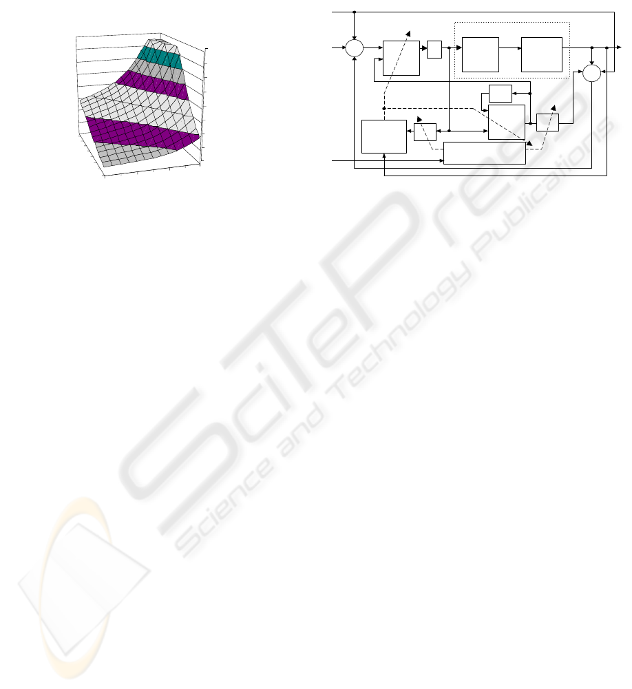
expected from equation 13. The relation between gas

flow and the delta temperature presents a weak but

important non-linearity for a specific water flow.

However, the relation between water flow and the

delta water temperature presents a strong non-

linearity for a specific gas flow.

The gas water heater plant presents a variant time

delay. The variation of the time delay function td(t)

depends mainly on the velocity of the water inside of

the tubes in the permutation chamber. The time-

delay approximation function td(k) for the one

second sampled system is illustrated in equation 15.

⎪

⎩

⎪

⎨

⎧

<≤

≥

l/min 3,5wf(k)if (sec)5

l/min 9,5wf(k)3,5if (sec)4

l/min 9,5 wf(k)if (sec)3

td(k)

(15)

5.2 ASPC specific structure and on-

line model identification

From empirical knowledge, heating systems are

usually first order systems plus a time delay, based

in this knowledge the dynamic linear part of the

NFHM will be considered a first order dynamic

function. Therefore, the dynamic linear model

function is expressed in equation 16.

td)-gf(k offunction linear -onntd)-nlgf(k

td)-nlgf(kb1)-t(kat(k)

+∆=∆

(16)

The non-linear gas flow nlgf(.) corresponds to the

f(.) non-linear function in the NFHM.

The ASPC is implemented in two steps: first, off-

line estimation of the non-linear static parameters

and second, on-line identification of the linear

dynamic parameters updating the direct and inverse

models of the plant, as illustrated in figure 7.

The Time-Delay Approximation Function updates

on-line the time delay approximation as expressed in

equation 15 and illustrated in figure 7.

40,0

60,0

80,0

100,0

14,5

12,7

10,9

9,0

7,2

5,3

3,5

2,0

22,0

42,0

62,0

82,0

Delta Temperature

(ºC)

Gas

Flow

(%)

Water Flow (l/min)

Static Gas Water Heater Surface

20,0

Figure 6: Static characterization of the gas water

heater

Plant

r(k)

-1

hwt(k)lgf(k)

-1

(.)

gf(k)

-1

(z)

"Linearization" of the plant

e(k)

RLS

with

RCM

-td (k)

cwt(k)

∆t(k)-e(k)

-td (k)

G(z)

wf(k)

Time Delay

Approximation Function

Figure 7: ASPC for the gas water heater.

In this particular example the variable water flow,

changes the time constant and the static gain of the

system. Therefore, this static gain should be taking

into account in the non-linear static function

parameters calculation. The non-linear static

parameters were calculated with a constant water

flow of 9 l/m that gives a static gain of 0.873 (see

training signal). The non-linear static function

parameters calculated in (Vieira

el at. 2004b) should

be multiplied by the inverse of this particular static

gain therefore this non-linear static parameters will

be general for all water flow range.

First step is the non-linear static inverse function

parameters identification off-line. It was used a zero-

order TS fuzzy model implemented with three bell

shaped fuzzy sets that impose three simple rules.

With input universes of discourse normalized and

using the training and test data sets used in the

NFHM approach exposed in (Vieira

el at., 2004b)

the zero-order TS fuzzy model parameters are:

=0.274, bb

=1.614, cc

=-0.023, d

=0.1717,

=0.352, bb

=2.060, cc

=0.515, d

=0.666,

=0.407, bb

=2.125, cc

=1.008 and d

=1.249.

After the non-linear static inverse function

parameters calculus the initial linear parameters are

calculated using the LS algorithm. The initial linear

dynamic identification parameters found are

=0.790 and b

=0.210.

Finally, iteration-by-iteration, the linear dynamic

parameters are recalculated, updating the proposed

ASPC based in NFHMs.

ADAPTIVE SMITH PREDICTIVE CONTROL OF NON-LINEAR SYSTEMS USING NEURO-FUZZY

HAMMERSTEIN MODELS

5.3 Comparative results using the

ASPC and SPMSPC

For the comparison of the two controllers, ASPC

and SPMSPC, the references hot water temperature

and water flow variables were applied and the

respective mean square errors (MSE) were

calculated r(k-td)-y(k). It was used r(k-td) to avoid

the error introduced by the time delay. The final

results are expressed in table 1.

0 100 200 300 400 500 600 700 800 900 1000

r and hwt (ºC)

0 100 200 300 400 500 600 700 800 900 1000

100

gf (%)

0 100 200 300 400 500 600 700 800 900 1000

wf(l/min)

0 100 200 300 400 500 600 700 800 900 1000

-10

Time(seconds)

e (ºC)

0 100 200 300 400 500 600 700 800 900 1000

-10

r-hwt (ºC)

Figure 8: ASPC results

0 100 200 300 400 500 600 700 800 900 1000

Table 1: Mean square errors of the two controllers

Algorithm MSE

ASPC 1.858

SPMSPC 1.953

As can be seen from the results both architectures

ASPC and SPMSPC achieve good results. But the

SPMSPC approach is not an adaptive model

controller approach, therefore, it can be seen in

Figure 9 that there is an error between the direct

model and the real plant. The cause that is

responsible for the difference between the model and

the plant is called load. This load induced a worst

control performance.

The ASPC approach is an adaptive model

controller approach, therefore, it can be seen in

Figure 8 that there is no load in the system.

However, the control results are affected by the

tuning time and variation of the linear parameters.

In Figure 10 it can be seen that the linear dynamic

parameters are similar in both controllers. The small

differences observed became from the possible non-

optimal parameters achieved with the genetic

algorithms in the SPMSP and from the on-line

adaptation of the linear dynamic parameters with a

continues variation of the time delay that was

approximated to the discrete time by equation 15.

6 CONCLUSIONS AND FUTURE

WORK

This work presents a new model based Smith

predictive adaptive controller using Hammerstein

neuro-fuzzy model identification. It presents a new

and simple method for the neuro-fuzzy Hammerstein

model on-line identification and its generalisation.

The NFHM approach uses a zero-order Takagi-

Sugeno fuzzy model to approximate the non-linear

static function that is tuned off-line using gradient

decent algorithm and to identify the linear dynamic

function it is used the Recursive Least Square on-

line estimation with Covariance Matrix Reset

(RLSCMR). The CMR algorithm is used for a faster

convergence of the identified parameters because if

the load presents big changes the parameters should

r and hwt (ºC)

0 100 200 300 400 500 600 700 800 900 1000

100

gf (%)

0 100 200 300 400 500 600 700 800 900 1000

wf(l/min)

0 100 200 300 400 500 600 700 800 900 1000

-10

Time(seconds)

e (ºC)

0 100 200 300 400 500 600 700 800 900 1000

-10

r-hwt (ºC)

Figure 9: SPMSPC results

0 100 200 300 400 500 600 700 800 900 1000

0.1

0.2

0.3

0.4

0.5

0.6

0.7

0.8

0.9

Linear Parameters - a1 b0

Time(seconds)

Figure 10: On-line parameters variation.

(

ASPC continues line and SPMSPC dot line

)

ICINCO 2004 - SIGNAL PROCESSING, SYSTEMS MODELING AND CONTROL

have a fast and stable change too, maintaining the

robustness of the controller.

Finally, the proposed ASPC and SPMSPC control

approaches were successful applied to an illustrative

example: gas water heater system. The ASPC

achieve better control results than the SPMSPC

because, even when the load (water flow / maximum

power) changes the dynamic of the system, the

linear parameters will adapt then selves. The

SPMSPC was optimise for a fixed maximum power

so if the maximum power changes the control results

will be worse than the ones achieved with the ASPC.

REFERENCES

Abonyi J., Babuska R., Botto M., Szeifert F., Nagy L.

2000. Identification and Control of Non-linear

Systems Using Fuzzy Hammerstein Models. Industrial

Engineering and Chemistry Research , vol. 39, no. 11,

pp. 4302-4314.

Abonyi J., Nagy L., Szeifert F., 1999. Adaptive Fuzzy

Inference System and its Application in Modelling and

Model Based Control

, Chemical Engineering Research

and Design, vol. 77A, pp. 281-290.

Abonyi J., Bódizs A., Nagy L., Szeifert F., 2000b. Hybrid

Fuzzy Convolution Model and its Application in

Model Predictive Control, Chemical Engineering

Research and Design, vol. 78(A), pp. 597-604.

Fink A., Nelles O., Fischer M. and Isermann R., 2001.

Nonlinear Adaptive Control of a Heat Exchanger,

International Journal of Adaptive Control and Signal

Proc., vol. 15(8), pp. 883-906.

Potmann M., Seborg D. 1997. A Nonlinear Predictive

Control Strategy Based on Radial Basis Function

Models

, Computers Chemistry Engineering, vol. 21

(9), pp. 965-980.

Tan Y., Nazmul Karim M., 2002. Smith Predictor Based

Neural Controller with Time Delay Estimation,

Proceedings of 15th Triennial World Congress, IFAC.

Tan Y., Cauwenberghe A., 1999. Neural Network Based d

steps ahead Predictors for Non-Linear Systems with

Time Delay, Engineering Applications of Artificial

Intelligence, vol. 12(1), pp. 21-35.

Vieira J., Mota A., 2003. Smith Predictor Based Neural

Fuzzy Controller Applied in a Water Gas Heater that

Presents a Large Time-Delay. Proceedings of IEEE

International Conference on Control Application, vol.

1, pp. 362-367.

Vieira J., Mota A., 2004a. Water Gas Heater Non-Linear

Physical Model: Optimisation with Genetic

Algorithms. Proceedings of IASTED 23

International

Conference on Modelling, Identification and Control,

February 23-25, vol. 1, pp. 122-127.

Vieira J., Mota A., 2004b. Parameter Estimation of Non-

Linear Systems with Hammerstein Models Using

Neuro-Fuzzy and Polynomial Approximation

Approaches, Proceedings International Conference on

Fuzzy Systems IEEE-FUZZ 2004, July 25-29,

(accepted).

ADAPTIVE SMITH PREDICTIVE CONTROL OF NON-LINEAR SYSTEMS USING NEURO-FUZZY

HAMMERSTEIN MODELS