
MODELLING AND PERFORMANCE EVALUATION OF DES
— A MAX-PLUS ALGEBRA TOOLBOX FOR MATLAB
Jarosław Sta
´
nczyk
Lehrstuhl f
¨
ur Systemtheorie technischer Prozesse, Otto-von-Guericke University Magdeburg
Postfach 41 20, D-39016 Magdeburg, Germany
Eckart Mayer
Max Planck Institute Dynamics of Complex Technical Systems, Sandtorstr. 1, D-39106 Magdeburg, Germany
J
¨
org Raisch
Lehrstuhl f
¨
ur Systemtheorie technischer Prozesse, Otto-von-Guericke University Magdeburg
Postfach 41 20, D-39016 Magdeburg, Germany
and Max Planck Institute Dynamics of Complex Technical Systems, Sandtorstr. 1, D-39106 Magdeburg, Germany
Keywords:
Discrete event systems, max-plus algebra, performance evaluation.
Abstract:
This paper discusses the usefulness of (max, +) algebra as a mathematical modelling framework for discrete
event systems (DESs). A Max-Plus Algebra Toolbox developed at Lehrstuhl f
¨
ur Systemtheorie technischer
Prozesse is presented. This software package is a set of functions to take advantage of the (max, +) algebra
in the Matlab environment for rapid prototyping, design, and analysis of DESs. An overview of the modelling
and analysis concepts of the (max, +) algebra approach for DES is given. Application examples are provided
in the final part of the paper to illustrate the potential of this approach and the toolbox.
1 INTRODUCTION
Many phenomena from manufacturing systems,
telecommunication networks and transportation sys-
tems can be described as so-called discrete event
systems (DES), or discrete event dynamic systems.
A DES is a dynamic asynchronous system where the
state transitions are initiated by events that occur at
discrete instants of time. An event corresponds to the
start or the end of an activity. A common property of
such examples is that the start of an activity depends
on termination of several other activities. Such sys-
tems cannot conveniently be described by differential
or difference equations, and naturally exhibit a peri-
odic behaviour.
An introduction to DES has been given, e.g. in
(Cassandras and Lafortune, 1999). Many frameworks
exist to study DES. Examples are queuing theory,
e.g. (Gross and Harris, 1997), Petri nets, e.g. (Ba-
naszak et al., 1991), the (max, +) algebra (Baccelli
et al., 1992) and many others. The most widely used
technique to analyze DES is computer simulation.
An important drawback of simulation is that it often
does not give a real understanding of how parame-
ter changes affect important system properties such
as stability, robustness and optimality of system per-
formance. Analytical techniques can provide a much
better insight in this respect. Therefore, formal meth-
ods are to be preferred as tools for modelling, analysis
and control of DES.
This paper presents a software tool for rapid pro-
totyping, design and analysis of DESs: a Max-Plus
Algebra Toolbox for Matlab (Sta
´
nczyk, 2003). This
is a set of functions implementing major aspects of
the (max, +) algebra in the Matlab environment.
The (max, +) algebra was first introduced in
(Cuningham-Green, 1979). A standard reference is
(Baccelli et al., 1992), a brief survey of methods and
applications of this algebra is given in (Cohen et al.,
1999) and (Gaubert and Max-Plus, 1997). In certain
aspects, the (max, +) algebra is comparable to the
conventional algebra. In the (max, +) algebra the
addition (+) and multiplication (×) operators from
the conventional algebra are replaced by the maxi-
mization (max) and addition (+) operators, respec-
tively. Using these operators, a linear description (in
the (max, +) algebra sense) of certain non-linear sys-
tems (in the conventional algebra) is achieved.
There are other tools available in the Internet for
computation in (max, +) algebra:
269
Sta
´
nczyk J., Mayer E. and Raisch J. (2004).
MODELLING AND PERFORMANCE EVALUATION OF DES — A MAX-PLUS ALGEBRA TOOLBOX FOR MATLAB.
In Proceedings of the First International Conference on Informatics in Control, Automation and Robotics, pages 270-275
Copyright
c
SciTePress

• the MaxPlus Toolbox for Scilab (INRIA Max-
Plus Working Group, 1998);
• MAX: a Maple package (Gaubert, 1992).
This contribution is organized as follows. In
Section 2, the (max, +) algebra formalism and the
(max, +) state space description of DESs are intro-
duced. The Max-Plus Algebra Toolbox for Matlab is
shortly described in Section 3. Section 4 is devoted
to illustrate the potential and abilities of the presented
tool. In the last section, we summarize the paper and
indicate some directions for future research.
2 MAX-PLUS ALGEBRA
In this section, we give an introduction to the
(max, +) algebra. Most of the material presented
in this section is taken from (Baccelli et al., 1992)
and (Cuningham-Green, 1979), where a complete
overview of the (max, +) algebra can be found. We
also present the state space description of DES.
2.1 Max-plus algebra
(max, +) algebra is defined as follows:
• R
ε
= R ∪ {ε}, where R is the field of real numbers
and ε = −∞;
• ∀a, b ∈ R
ε
: a ⊕ b = max(a, b);
• ∀a, b ∈ R
ε
: a ⊗ b = a + b.
The algebraic structure R
max
= (R
ε
, ⊕, ⊗, ε, e), e =
0,is called the max-plus algebra. More specifically,
the algebraic structure R
max
is an idempotent, com-
mutative semiring (or diod). This structure satisfies
all the semiring axioms, i.e.:
• commutativity of operation ⊕:
∀a, b ∈ R
ε
: a ⊕ b = b ⊕ a;
• associativity of operation ⊕:
∀a, b, c ∈ R
ε
: (a ⊕ b) ⊕ c = a ⊕ (b ⊕ c);
• existence of a neutral element (ε) for operation ⊕:
∀a ∈ R
ε
: a ⊕ ε = ε ⊕ a = a;
• associativity of operation ⊗:
∀a, b, c ∈ R
ε
: (a ⊗ b) ⊗ c = a ⊗ (b ⊗ c);
• existence of a neutral element (e) for operation ⊗:
∀a ∈ R
ε
: e ⊗ a = a ⊗ e = a;
• ε is absorbing for ⊗:
∀a ∈ R
ε
: a ⊗ ε = ε;
• distributivity of ⊗ with respect to ⊕:
∀a, b, c ∈ R
ε
: a ⊗ (b ⊕ c) = (a ⊗ b) ⊕ (a ⊗ c),
(b ⊕ c) ⊗ a = (b ⊗ a) ⊕ (c ⊗ a).
This semiring is:
• commutative with regard to ⊗:
∀a, b ∈ R
ε
: a ⊗ b = b ⊗ a;
• idempotent:
∀a ∈ R
ε
: a ⊕ a = a;
Note that non-zero elements do not have an inverse
for ⊕, because a ⊕ x = ε does not have a solution for
a 6= ε.
We will write ab for a ⊗ b whenever there is no pos-
sible confusion. Now, we extend the max-plus alge-
bra operations to vectors and matrices in the following
way.
The (max, +) sum of a scalar a ∈ R
ε
and a vector
b = (b
i
) ∈ R
n
ε
is defined by:
(a ⊕ b)
i
= a ⊕ b
i
, i = 1, . . . , n. (1)
The sum ⊕ of matrices A = (a
ij
), B = (b
ij
) ∈
R
m×n
ε
is defined to be the m × n matrix A ⊕ B ob-
tained by adding corresponding entries. That is,
(A ⊕ B)
ij
= a
ij
⊕ b
ij
,
i = 1, . . . , m; j = 1, . . . , n. (2)
We define the product of a scalar a ∈ R
ε
and a vector
b = (b
i
) ∈ R
n
ε
by:
(a ⊗ b)
i
= a ⊗ b
i
, i = 1, . . . , n. (3)
The product ⊗ of matrices A = (a
ik
) ∈ R
m×p
ε
and
B = (b
kj
) ∈ R
p×n
ε
is defined to be the m × n matrix
whose (i, j)-entry is the inner product of the i
th
row
of A with the j
th
column in B. That is,
(A ⊗ B)
ij
=
p
M
k=1
a
ik
⊗ b
kj
= max
k
(a
ik
+ b
kj
),
i = 1, . . . , m; j = 1, . . . , n, (4)
where:
m
M
j=1
a
j
is short-hand for a
1
⊕ · · · ⊕ a
m
.
The matrix I
n
= (e
ij
) ∈ R
n×n
ε
with e’s on the main
diagonal and ε’s elsewhere is called the identity ma-
trix of order n.
The matrix ε = (ε
ij
) ∈ R
m×n
ε
with ε
ij
= ε for all
i, j, is the zero-matrix.
The operator
∗
for square matrices A ∈ R
n×n
ε
is de-
fined by:
A
∗
=
M
k∈N
0
A
k
, (5)
where: A
0
= I
n
, A
k
= A ⊗ A
k−1
and N
0
is the
set of nonnegative integers. (5) is only meaningful if
the right hand side converges.
2.2 State space description of timed
event graph
Timed event graphs are (timed) Petri-nets, which are
convenient to model (timed) synchronization prob-
lems. They are characterized by the fact that every
place has exactly one predecessor transition and one
successor transition. Time constraints are modelled
by so-called holding times, representing the minimum
amount of time a token has to “spend” in a place be-
fore it can contribute to enable a “downstream” tran-
sition.
Let x
i
(k) denote the time instant, when an “internal”
transition i can fire for the k
th
time, and x(k) =
(x
i
(k)) the corresponding vector of firing times. Sim-
ilarly, let u
i
(k) denote the firing times of “input tran-
sitions” which can be triggered by the outside world,
and y
i
(k) the firing times of “output transitions”
which carry information to the outside world. It is
then straightforward, to read the following (max, +)
equations from the timed event graph:
x(k +1) =
M
M
i=0
A
i
x(k +1−i)⊕
N
M
j=0
B
j
u(k +1−j),
(6)
y(k) =
M
M
i=0
C
i
x(k − i) ⊕
N
M
j=0
D
j
u(k − j). (7)
If A
?
0
exists, by defining a state vector
e
x(k) = [
x
0
(k) x
0
(k − 1) . . . x
0
(k − M )
]
0
,
(8)
an augmented input vector
e
u(k) = [
u
0
(k) u
0
(k − 1) . . . u
0
(k − N )
]
0
,
(9)
and matrices
e
A =
A
∗
0
A
1
A
∗
0
A
2
. . . . . . A
∗
0
A
M
I ε . . . . . . ε
ε
.
.
.
.
.
.
ε . . . ε I ε
, (10)
e
B =
A
∗
0
B
0
. . . A
∗
0
B
N
ε . . . ε
.
.
.
.
.
.
ε . . . ε
, (11)
e
C = [
C
0
. . . C
M
] , (12)
e
D = [
D
0
. . . D
N
] , (13)
where I and ε are appropriately sized (max, +)-
algebraic identity and zero matrices, respectively,
Eqns. (6), (7) can be written as
e
x(k + 1) =
e
A
e
x(k) ⊕
e
B
e
u(k + 1), (14)
e
y(k) =
e
C
e
x(k) ⊕
e
D
e
u(k). (15)
3 THE TOOLBOX
The Max-Plus Algebra Toolbox is a set of functions,
written as M-files, to take advantage of the (max, +)
algebra in the Matlab environment. This package has
been developed for fast and easy modelling and anal-
ysis of DESs amenable to (max, +) algebra. Basic
elements of this toolbox are:
• elementary functions: the (max, +) addition for
scalars, vectors and matrices, multiplication, rise to
a power, etc.;
• solving an equation of type x = Ax ⊕ b;
• solving an equation of type Ax = b;
• solving the spectral problem Ax = λx, i.e. deter-
mining the eigenvalue and eigenvectors of A;
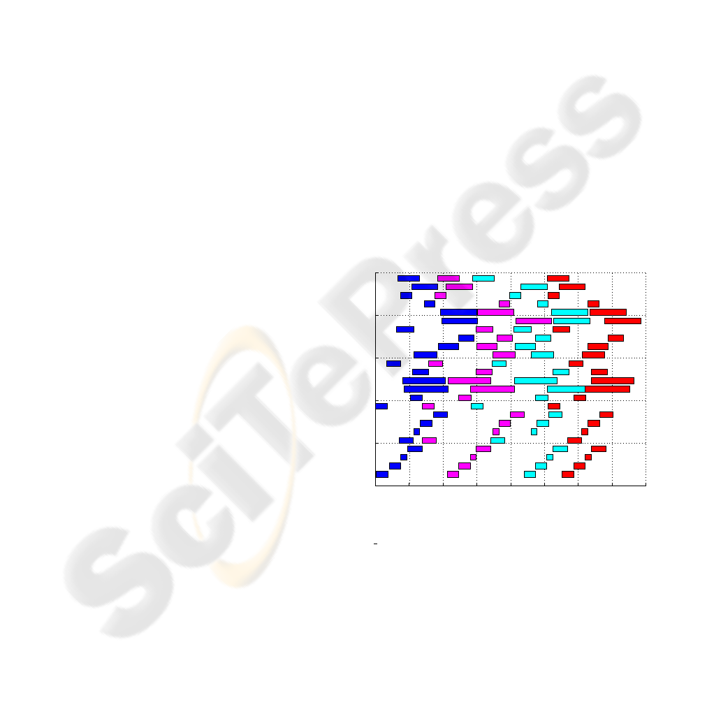
• DESs analysis:
– graphically by providing Gantt charts (see
Fig. 1),
– calculate performance indices (flow time, re-
source utilizations, etc.),
– calculate cycle time and length of transient state.
0 500 1000 1500 2000 2500 3000 3500 4000
0
5
10
15
20
25
time
events
Figure 1: An exemplary Gantt chart generated by the
mp
gantt() function.
4 APPLICATION
In order to illustrate our software package let us ex-
amine two examples: a simple manufacturing sys-
tem and a transportation system, namely the suburban
train network of Stuttgart, Germany.
4.1 Multi-product manufacturing
system
The idea for this example has been taken from (Bac-
celli et al., 1992). Consider a manufacturing system
that consists of three machines (M
1
, M
2
and M
3
).
In this manufacturing system three different types of
parts (P
1
, P
2
and P
3
) are produced according to a cer-
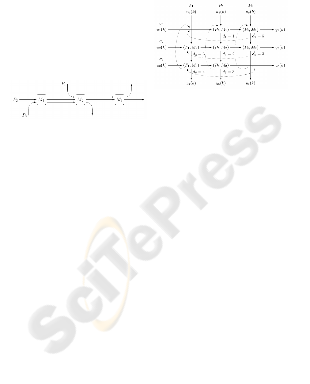
tain product mix. The routes followed by the various
types of parts are depicted in Fig. 2.
Figure 2: The routing of the various types of parts along the
machines.
Parts of type P
1
first visit machine M
2
and then go
to M
3
. Parts of type P
2
enter the system via machine
M
1
, then they go to machine M
2
and finally leave the
system through machine M
3
. Parts of type P
3
first
visit machine M
1
and then go to M
2
. It is assumed
that:
• Parts are carried around on pallets. There is one
pallet available for each type of part.
• It is assumed that the transportation times are neg-
ligible and that there are no set-up times on the ma-
chines when they switch from one part type to an-
other.
• The sequencing of the various parts on the ma-
chines is known: on machine M
1
it is (P
2
, P
3
),
i.e. the machine first processes a part of type P
2
and then a part of type P
3
, on machine M
2
the se-
quence is (P
1
, P
2
, P
3
), and (P
1
, P
2
) on machine
M
3
. We will call these sequences local dispatching
rules and we will describe them as σ (i.e. σ
1
for the
sequence on M
1
, σ
2
for the sequence on M
2
, and
σ
3
for M
3
).
The information about the sequencing and the du-
ration of the various activities (processing times) is
shown in Fig. 3. In this figure, the activities are repre-
sented by ordered pairs of the form (P
i
, M
j
) mean-
ing that a part of type P
i
is processed on machine
M
j
. The arcs represent the precedence constraints be-
tween activities. At the bottom right of each activity
we have indicated its duration, e.g. (P
1
, M
2
) (activity
3) has duration d
3
= 3.
In order to simplify the process of deriving the evo-
lution equations of this system, we shall first look at
what happens in one cycle of the production process.
We define:
Figure 3: The sequence and the duration of the various ac-
tivities.
• u
i
(k) — time instant at which machine M
i
is avail-
able for the first activity that should be performed
on it in the k
th
production cycle for i = 1, 2, 3;
• u
j
(k) — time instant at which the raw material for
a part of type P
j−3
is available in the k
th
produc-
tion cycle for j = 4, 5, 6;
• x
i
(k) — time instant at which activity i starts in the
k
th
production cycle for i = 1, 2, . . . , 7;
• y
i
(k) — time instant at which machine M
i
has fin-
ished processing the last part of the k
th
production
cycle that should be processed on it for i = 1, 2, 3.
• y
j
(k) — time instant at which the finished product
of type P
j−3
of the k
th
production cycle has been
completed for j = 4, 5, 6;
We have the following evolution equations:
x
1
(k + 1) = 5x
2
(k) ⊕ 3x
7
(k)
⊕u
1
(k + 1) ⊕ u
5
(k + 1),
x
2
(k + 1) = 1x
1
(k + 1) ⊕ 3x
5
(k)
⊕u
6
(k + 1), (16)
.
.
.
or, more compactly:
x(k + 1) = A
0
x(k + 1) ⊕ A
1
x(k)
⊕B
0
u(k + 1),
= Ax(k) ⊕ Bu(k + 1), (17)
where A = A
∗
0
A
1
, and B = A
∗
0
B
0
.
An exemplary analysis of the considered system
based on the Max-Plus Algebra Toolbox is shown be-
low. It provides cycle time and consecutive states
(x(k)) of the system. It is assumed that x(0) =
[ε]
7×1
, i.e. all machines are idle in the beginning,
and u(1) = [e]
6×1
, i.e. all machines can be started
without delay.

% definitions of matrices:
A0 = [
-inf -inf -inf -inf -inf -inf -inf
1 -inf -inf -inf -inf -inf -inf
-inf -inf -inf -inf -inf -inf -inf
1 -inf 3 -inf -inf -inf -inf
-inf 5 -inf 2 -inf -inf -inf
-inf -inf 3 -inf -inf -inf -inf
-inf -inf -inf 2 -inf 4 -inf ]
A1 = [
-inf 5 -inf -inf -inf -inf 3
-inf -inf -inf -inf 3 -inf -inf
-inf -inf -inf -inf 3 4 -inf
-inf -inf -inf -inf -inf -inf -inf
-inf -inf -inf -inf -inf -inf -inf
-inf -inf -inf -inf -inf -inf 3
-inf -inf -inf -inf -inf -inf -inf ]
B0 = [ 0 -inf -inf -inf 0 -inf
-inf -inf -inf -inf -inf 0
-inf 0 -inf 0 -inf -inf
-inf -inf -inf -inf -inf -inf
-inf -inf -inf -inf -inf -inf
-inf -inf 0 -inf -inf -inf
-inf -inf -inf -inf -inf -inf ]
% create the A matrix
>> A = mp_multi(mp_star(A0),A1);
% calculate a cycle time
>> lambda = mp_mcm(A)
lambda =
9.5000
% create the B matrix
>> B = mp_multi(mp_star(A0),B0);
% determine initial conditions
>> x = mp_zeros(7,1);
>> u = mp_ones(6,1);
% calculate a sequence of a state vector
>> X(:,1) =
mp_sum(mp_multi(A,x),mp_multi(B,u));
>> for i=2:6
X(:,i) = mp_sum(mp_multi(A,X(:,i-1)),
mp_multi(B,u));
end
>> X
X =
0 10 19 29 38 48
1 11 20 30 39 49
0 9 19 28 38 47
3 12 22 31 41 50
6 16 25 35 44 54
3 12 22 31 41 50
7 16 26 35 45 54
4.2 Transportation system
Max-plus algebra has been intensely used in mod-
elling and analysis of train traffic networks, i.e.
(Braker, 1993). As an application example, a model
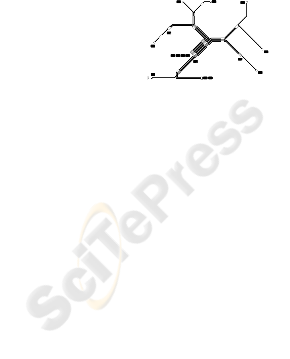
for the suburban train network of Stuttgart, Germany,
is briefly described in this section. The structure of
the network is pictured in Fig.4. As short followup
times of trains and single line track segments (used in
both directions) are critical features of this transporta-
tion system, a specifically detailed max-plus model
has been used for analysis and simulation. In addi-
tion to passenger changeover times also safety con-
straints for track segments used consecutively by sev-
eral trains are taken into account in order to get an
accurate model.
Generally, the max-plus state space model structure
as given in (14)–(15) is used. The state vector is com-
posed of the event times for the following types of
events:
• departure of trains at terminal stations
• arrival resp. departure of trains at changeover sta-
tions
• trains entering track segments shared with other
lines
• trains entering resp. leaving single track segments
The dependencies between the events (entries in
matrix A
0
resp. A
1
) are
• minimum travelling times of trains including
stopover at intermediate stations and minimum
turnaround times at endpoints of lines
• minimum times passengers need for changeover
between trains
• minimum followup time distance for consecutive
trains on the same track
• safety constraints for single track segments shared
by trains moving in opposite directions
In addition to the standard max-plus model (14), a
timetable is needed for cyclically operated transporta-
tion systems. Timetable information consists of two
parts: the cycle time and the timetable vector w
0
. For
the current example, cycle time is T = 30: under nor-
mal conditions, operation is repeated every 30 min-
utes. The location of trains at any time t is identical
to the location at time t − 30 with the only difference
that all trains have moved forward by one position on
their line. The timetable vector w
0
provides the earli-
est time instant at which any event is allowed to hap-
pen. The k
th
occurrence of any event is not allowed
to happen before the time given by the timetable:
x(k) ≥ w(k) = w
0
+ k · T . (18)
Thus, the timetable enters the state space model as an
input u with B = I and u(k) = w(k) = w
0
⊗ T
k
.
For the suburban train network of Stuttgart, an
overall number of 73 events is necessary. The system
matrix A is determined from A
0
and A
1
as given in
Eqn. (17). Within A, the number of non-ε entries,
i.e. the number of timed dependencies between the
events is 426.
Hence, the overall max-plus algebra model for the
cyclically operated train track network is:
x(k + 1) = Ax(k) ⊕ w(k + 1) (19)
x(0) = x
0
with: w(k) = w
0
T
k
, x(k) ∈ R
73
ε
, A ∈ R
73×73
ε
.
The max-plus model (19) is used to analyze the
system. The eigenvalue for the system matrix A can
be calculated using the mp_egv1() command of the
max plus toolbox: λ = 26. The eigenvalue repre-
sents the minimum possible cycle time of the sys-
tem. Thus, with the number of trains and the times
as given, the system could be operated under a cycle
time of 26 minutes. Comparing the timetable cycle
time of T = 30 minutes and the eigenvalue, we find a
stability margin of 4 minutes per cycle, which allows
for diminishing of delays.
A brief example illustrates simulation of the max-
plus model. In simulation, the time instants for the
events of the system, i.e. x(1), x(2), . . . are calcu-
lated based on the vector of initial times x(0) =
x
0
. For normal operation, the vector of initial times
matches the timetable vector: x(0) = w
0
. In or-
der to investigate the effects of a traffic disruption,
the system can instead be simulated starting from an
initial vector where one or more time values are in-
creased compared to the timetable vector. In our ex-
ample, the value for the event time of a train leav-
ing Herrenberg station is increased by 7 time units.
The state sequence x(1), x(2), . . . can now be calcu-
lated iteratively. The deviation from the timetable,
z(k) = x(k) − w(k), can then be determined. As
a measure for the ability of the system to cope with
this type of disruption, one is especially interested in
the number of cycles that are necessary for the de-
lays to vanish entirely. For the given example, this
is the case after 3 cycles, i.e. x(k) = w(k), k ≥ 3.
Fig.4 shows qualitatively the effects of the disruption
spreading over the network during the first 3 cycles.
The affected stops are shown in gray.
5 CONCLUDING REMARKS
In this paper, a software package for modelling and
performance evaluation of DESs in the (max, +) al-
gebra has been presented. The implementation at this
moment is more than tentative, so every remark and
suggestion is welcome. The tool is available via the
Internet. A brief manual, in which all functions and
algorithms used in the toolbox are described is also
available. The tool is still under development and ad-
ditional functions will be added.
Freiberg
a. N.
Bad
Cannstatt
S3
S1
S6
S4 S5 S6
S6
S1
S1
S6
S2
S4
S1
Leonberg
Ludwigsburg
Renningen
Waiblingen
Rohr
Zuffenhausen
S3
S2
S5
Backnang
Weil der Stadt
Hauptbahnhof
Flughafen
Marbach
Bietigheim
Schwabstrasse
Esslingen
Plochingen
Schorndorf
Herrenberg
7
Figure 4: Railway network map with delays.
REFERENCES
Baccelli, F., Cohen, G., Olsder, G., and Quadrat, J.-P.
(1992). Synchronisation and Linearity: An Algebra
for Discrete Event Systems. John Wiley & Sons, Inc.,
Chichester, England.
Banaszak, Z., Jampolski, L., Hasegawa, K., Krogh, B.,
Takahasi, K., and Borusan, A. (1991). Modelling and
Control of FMS. Petri Net Approach. Wroclaw Uni-
versity of Technology, Wrocław, Poland.
Braker, J. G. (1993). Algorithms and Applications in Timed
Discrete Event Systems. PhD thesis, Department of
Technical Mathematics and Informatics, Delft Univer-
sity of Technology, Delft.
Cassandras, C. and Lafortune, S. (1999). Introduction to
Discrete Event Systems. Kluwer Academic Publish-
ers, Boston, USA.
Cohen, G., Gaubert, S., and Quadrat, J.-P. (1999). Max-plus
algebra and system theory: where we are and where to
go now. Annual Reviews in Control, 23(1):207–219.
Cuningham-Green, R. (1979). Minimax Algebra, volume
166 of Lecture Notes in Economics and Mathematical
Systems. Springer Verlag, Berlin, Germany.
Gaubert, S. (1992). MAX: a Maple package for
the (max,+) algebra. Available in the Internet:
http://amadeus.inria.fr/gaubert/.
Gaubert, S. and Max-Plus (1997). Methods and applications
of (max,+) linear algebra. Technical Report 3088, IN-
RIA, Rocquencourt, France.
Gross, D. and Harris, C. (1997). Fundamentals of Queueing
Theory. John Wiley & Sons, Inc., 3 edition.
INRIA MaxPlus Working Group (1998). MaxPlus
Toolbox for Scilab. Available in the Internet:
http://www.maxplus.org.
Sta
´
nczyk, J. (2003). Max-Plus Algebra Tool-
box for Matlab. Available in the Internet:
http://ifatwww.et.uni-magdeburg.de/.
