
A STOCHASTIC OFF LINE PLANNER OF OPTIMAL DYNAMIC
MOTIONS FOR ROBOTIC MANIPULATORS
Taha Chettibi, Moussa Haddad, Samir Rebai
Mechanical Laboratory of Structures, EMP, B.E.B., BP17, 16111, Algiers, Algeria
Abd Elfath Hentout
Laboratory of applied mathematics, EMP, B.E.B., BP17, 16111, Algiers, Algeria
Keywords: Robotic manipulator, Motion planning, Sto
chastic optimization, Obstacles avoidance.
Abstract:
We propose a general and simple method that handles free (or point-to-point) motion planning problem for
redundant and non-redundant serial robots. The problem consists of linking two points in the operational
space, under constraints on joint torques, jerks, accelerations, velocities and positions while minimizing a
cost function involving significant physical parameters such as transfer time and joint torque quadratic
average. The basic idea is to dissociate the search of optimal transfer time T from that of optimal motion
parameters. Inherent constraints are then easily translated to bounds on the value of T. Furthermore, a
stochastic optimization method is used which not only may find a better approximation of the global
optimal motion than is usually obtained via traditional techniques but that also handles more complicated
problems such as those involving discontinuous friction efforts and obstacle avoidance.
1 INTRODUCTION
Motion planning constitutes a primordial phase in
the process of robotic system exploitation. It is a
challenging task because the robot behaviour is
governed by highly non linear models and is
subjected to numerous geometric, kinematic and
dynamic constraints (Latombe, 1991) (Angeles,
1997) (Chettibi, 2001). Two categories of motions
can be distinguished (Angeles, 1997) (Chettibi,
2000). The first covers motions along prescribed
geometric path and correspond, for example, to
continuous welding or glowing operations (Bobrow,
1985) (Kang, 1986) (Pfeiffer, 1987) (Chettibi,
2001b). The second, which is the focus of this
paper, concerns point-to-point (or free) motions
involved, for example, in discrete welding or pick-
and-place operations (Bessonnet, 1992) (Mitsi,
1995) (Lazrak, 1996) (Danes, 1998) (Chettibi,
2001a). In general, many different ways are
possible to perform the same task. This freedom of
choice can be exploited judiciously to optimize a
given performance criterion. Hence, motion
generation becomes an optimization problem. It is
here referred to as the optimal free motion planning
problem (OFMPP).
In the specialized literature, various resolutions
m
ethods have been proposed to handle the OFMPP.
They can be grouped in two main families; namely:
direct and indirect methods (Hull, 1997) (Betts,
1998). The indirect methods are, in general,
applications of optimal control theory and in
particular Pontryagin Maximum Principle (PMP)
(Pontryagin, 1965). Optimality conditions are stated
under the form of a boundary value problem that is
generaly too difficult to solve (Bessonnet, 1992)
(Lazrak, 1996) (Chettibi, 2000). Several techniques,
such as the phase plane method (Bobrow, 1985)
(Kang, 1986) (Jaques, 1986) (Pfeiffer, 1987), exploit
the structure only of the optimal solution given by
PMP and get numerical solutions via other means.
In general, such techniques are applied to limited
cases and have several drawbacks resumed below:
Th
ey require the solution of a N.L multi-point
shooting problem (David, 1997) (John, 1998 ),
They re
quire analytical computing of gradients
(Lazrak, 1996) (Bessonnet, 1992),
121
Chettibi T., Haddad M., Rebai S. and Hentout A. (2004).
A STOCHASTIC OFF LINE PLANNER OF OPTIMAL DYNAMIC MOTIONS FOR ROBOTIC MANIPULATORS.
In Proceedings of the First International Conference on Informatics in Control, Automation and Robotics, pages 121-128
DOI: 10.5220/0001132301210128
Copyright
c
SciTePress

The region of convergence may be small
(Chettibi, 2001) (Lazrak, 1996),
Path inequality are difficult to handle (Danes,
1998),
They introduce new variables known as co-state
variables that are, in general, difficult to estimate
(Lazrak, 1996) (Bessonnet, 1992) (Danes, 1998)
(Pontryagin, 1965).
In minimum time transfer problems, they lead to
discontinuous controls (bang-bang) that may
create many practical problems (Ola, 1994)
(Chettibi, 2001a). In fact, the controller must
work in saturation for long periods. The optimal
control leaves no control authority to compensate
for any tracking error caused by either unmodeled
dynamics or delays introduced by the on-line
feedback controller
To overcome these difficulties, direct methods have
been proposed. They are based on discretisation of
dynamic variables (states, controls). They seek to
solve directly a parameter optimization problem.
Then, N.L. programming (Tan, 1988) (Martin, 1997)
(Martin, 1999) (Chettibi, 2001a) or stochastic
optimization techniques (Chettibi, 2002b) are
applied to compute optimal values of parameters.
Other ways of discretisation can be found in
(Richard, 1993) (Macfarlane, 2001). These
techniques suffer, however, from numerical
explosion when treating high dimension problems.
Although they have been used successfully to solve
a large variety of problems, techniques based on
N.L. programming (Fletcher, 1987) (David, 1997)
(Danes, 1998) (John, 1998) (Chettibi, 2000) have
two essential drawbacks:
They are easily attracted by local minima ;
They generally require information on gradiant and
hessian that are difficult to get analytically. In
addition, continuity of second order must be
ensured, while realistic physical models may
include some discontinuous terms (frictions).
In parallel to these methods, that take into
account both kinematics and dynamics aspects of the
problem, numerous pure geometric planners have
been proposed to find solutions for the simplified
problem that consists of finding only feasible
geometric paths (Piano movers problem) (Latombe,
1991) (Overmars, 1992) (Barraquand, 1992)
(Kavraki, 1994) (Barraquand, 1996) (Kavraki, 1996)
(Latombe, 1999) (Garber, 2002). In spite of this
simplification, the problem still remains quite
complex with exponential computational time in the
degree of freedom (d.o.f.). Of course, any extension
(presence of obstacles, for example) adds in
computational complexity. Even so, various
practical planners have been proposed. Reference
(Latombe, 1991) gives an excellent overview of
early methods (before 1991) such as: potential field,
cell decomposition and roadmap methods, some of
which have shown their limits. For instance, a
potential field based planner is quickly attracted by
local minima (Khatib, 1986) (Latombe, 1991)
(Barraquand, 1992). Cell decomposition methods
often require difficult and quite expensive geometric
computations and data structures tend to be very
large (Latombe, 1991) (Overmars, 1992). The key
issue for roadmap methods is the construction of the
roadmap. Various techniques have been proposed
that produce different sorts of roadmaps based on
visibility and Voronoi graphs (Latombe, 1991).
During the last decade, interest was given to
stochastic techniques to solve various forms of
optimal motion planning problems. In particular,
powerful algorithms were proposed to solve the
basic geometric problem. Probabilistic roadmaps
(PRM) or Probabilistic Path Planners (PPP) were
introduced in (Overmars, 1992) (Barraquand, 1996)
(Kavraki, 1994) (Kavraki, 1996) and applied
successfully to complex situations. They are
generally executed in two steps: first a roadmap is
constructed, according to a stochastic process, then
the motion planning query is treated. Due to the
power of this kind of schemes, many perspectives
are expected as shown in (Latombe, 1999).
However, there are few attempts to apply them to
solve the complete OFMPP. References (LaValle,
1998) (LaValle, 1999) propose the method of
Rapidly exploring Random Trees (RRTs) as an
extention of PPP to optimize feasible trajectories for
NL systems. Dynamic model and inherent
constraints are taken into account.
In (Chettibi, 2002a), we introduced a different
scheme using a sequential stochastic technique to
solve the OFMPP. We present here this simple and
versatile method and how it can be used to handle
complex situations involving both friction efforts
and obstacle avoidance.
2 PROBLEM STATEMENT
Let us consider a serial redundant or non-redundant
manipulator with n d.o.f.. Motion equations can be
derived using Lagrange's formalism or Newton-
Euler formalism (Dombre, 1988) (Angeles, 1997):
(
)
(
)()
τ
=++ qGqqQqqM
&&&
,
(1a),
q, and are respectively joints position, velocity,
acceleration vectors. M(q) is the inertia matrix.
Q(
) is the vector of centrifugal and Coriolis
forces in which joints velocities appear under a
q
&
q
&&
qq
&
,
ICINCO 2004 - INTELLIGENT CONTROL SYSTEMS AND OPTIMIZATION
122

quadratic form. G(q) is the vector of potential
forces and
τ
is the vector of actuator efforts.
In order to make the dynamic model more realistic,
we may introduce, for the i
th
joint, friction efforts as
follows:
)())(()())((
))(),(()())((
1
ttqsignFtqFtqG
tqtqQtqtqM
i
s
i
v
ii
i
n
j
jij
τ
=+++
+
∑
=
&&
&&&
(1b),
V
i
F
and are, respectively, sec and viscous
friction coefficients of the i
s
i
F
th
joint.
The robot is required to move freely from an initial
state P
i
to a final state P
f
, both of which are specified
in the operational space. In addition to solving for
τ
(t) and transfer time T, we must find the trajectory
defined by q(t) such as the initial and the final state
are matched, constraints are respected and a cost
function is minimized.
The cost function adopted here is a balance
between transfer time T and the quadratic average of
actuator efforts:
∫
∑
=
⎟
⎟
⎠
⎞
⎜
⎜
⎝
⎛
−
+=
T
n
i
max
i
i
obj
dt
)t(
TF
0
1
2
2
1
τ
τ
µ
µ
(2).
µ
is a weighting coefficient chosen from [0,1] and
according to the relative importance we would like
to give to the minimization of T or to the quadratic
average of actuator efforts. The case
µ =
1 corresponds to the optimal time free motion
planning problem.
Constraints that must be satisfied during the
entire transfer (0 ≤ t ≤ T) are summarized bellow:
for i = 1, …, n we have bounds on:
- Joint torques:
()
max
ii
t
ττ
≤ (3a);
- Joint jerks :
()
max
ii
qtq
&&&&&&
≤
(3b);
- Joint accelerations:
()
max
ii
qtq
&&&&
≤ (3c);
- Joint velocities:
()
max
ii
qtq
&&
≤ (3d);
- Joint positions:
()
max
ii
qtq ≤ (3e).
Of course, non-symmetrical bounds on the above
physical quantities can also be handled without any
new difficulty.
Relations (3a, b, c, d and e) traduce the fact that
not all motions are tolerable and that power
resources are limited and must be used rationally in
order to control correctly the robot dynamic
behavior. Also, since joint position tracking errors
increase with jerk, constraints (3b) are introduced to
limit excessive wear and hence to extend the robot
life-span (Latombe, 1991) (Piazzi, 1998)
(Macfarlane, 2001).
In the case where obstacles are present in the
robot workspace, motion must be planned in such a
way collision is avoided between links and
obstacles. Therefore, the following constraint has to
be satisfied :
C(q)=False (3f).
The Boolean function C indicates whether or not the
robot at configuration q is in collision with an
obstacle. This function uses a distance function
D(q) that supplies for any robotic configuration the
minimal distance to obstacles.
3 REFORMULATION OF THE
PROBLEM
The normalization of the time scale, initially used to
make the problem with fixed final time, is exploited
to reformulate the problem and to make it propitious
for a stochastic optimization strategy. Details are
shown bellow.
3.1 Scaling
We introduce a normalized time scale as follows:
T.xt
=
with (4).
[]
1,0∈x
Hereafter, we will use the prime symbol to indicate
derivations with respect to x :
(
)
(
)
,",'
2
2
dx
xqd
q
dx
xdq
q ==
()
3
3
'"
dx
xqd
q =
(5).
Relations (1a) and (1b) can be written as follows:
(1a)
⇒
()
iii
GH
T
x +=
2
1
ψ
(6a)
(1b)
⇒
)(
11
2
qsignFqF
T
GH
T
s
ii
v
iiii
′
+
′
++=
ψ
(6b)
where:
()
(
)
max
i
i
i
x
x
τ
τ
ψ
=
,
max
i
ij
ij
M
M
τ
=
,
max
i
i
i
Q
Q
τ
=
,
max
i
i
i
G
G
τ
=
, =
i
H
i
n
j
jij
QqM +
∑
=1
"
(7)
and:
max
i
v
i
v
i
F
F
τ
=
,
max
i
s
i
s
i
F
F
τ
=
(8)
A STOCHASTIC OFF LINE PLANNER OF OPTIMAL DYNAMIC MOTIONS FOR ROBOTIC MANIPULATORS
123

3.2 Cost function
With the previous notations, the cost function (2)
becomes without friction efforts:
⎟
⎠
⎞
⎜
⎝
⎛
++=
4
4
2
2
0
T
S
T
S
STF
obj
(9),
Where S
0
, S
2
and S
4
are given by:
()
∫
∑
∫
∑
∫
∑
=
=
=
−
=
−=
−
+=
1
0
1
2
4
1
0
1
2
1
0
1
2
0
2
1
1
2
1
dxHS
dxGHS
dxGS
n
i
i
n
i
ii
n
i
i
µ
µ
µ
µ
(10).
It must be noted that S
0
, S
2
and S
4
are real
coefficients that do depend on the joint evolution
profile q(x) but that do not depend on T. Also, S
0
and S
4
are always positive. Expression (9)
represents a family of curves whose general shape,
for any feasible motion, is shown in figure 1a. The
minimum of each of these curves is reached when T
takes on the value T = T
m
given by :
2/1
0
40
2
22
2
12
⎟
⎟
⎟
⎠
⎞
⎜
⎜
⎜
⎝
⎛
++
=
S
SSSS
T
m
(11).
If friction efforts are taken into account, we
introduce the following quantities:
qFK
v
ii
′
=
,
)(qsignFGG
s
iii
′
+=
(12)
The expression of (2) becomes then :
⎟
⎟
⎠
⎞
⎜
⎜
⎝
⎛
++++=
4
4
3
3
2
21
0
T
S
T
S
T
S
T
S
STF
obj
(13)
where:
()
∫
∑
∫
∑
∫
∑
∫
∑
∫
∑
=
=
=
=
=
−
=
−=
+
−
=
−=
−
+=
1
0
1
2
4
1
0
1
3
1
0
1
2
2
1
0
1
1
1
0
1
2
0
2
1
)1(
2
2
1
)1(
2
1
λ
µ
λµ
λ
µ
λµ
λ
µ
µ
dHS
dKHS
dGHKS
dGKS
dGS
n
i
i
n
i
ii
n
i
iii
n
i
ii
n
i
i
(14)
For a given profile q(x), (13) represents a family of
curves whose general shape is shown in figure 1b,
but now the asymptotic line intersects the time axis
at
. Furthermore, T
01
/SS - T =
m
has to be
computed numerically since (11) is no longer
applicable.
3.3 Effects of constraints
Constraints imposed on the robot motion will be
handled sequentially within the iterative process of
minimization described in the next section. Already,
we can group constraints into several categories
according to the stage of the iterative process at
which they will be handled.
3.3.a Constraints of the first category
In the first category, we have constraints that will
not add any restriction on the value of T. For
example, joint position constraints (3e) become:
(
)
[]
nixqxq
ii
,,11,0
max
K=∈∀≤ (15),
and those due to obstacles presence (3f) become :
C(q(x))=False
[]
1,0∈
∀
x
(16)
In both cases, only the joint position profiles q(x) are
determinant.
3.3.b Constraints of second category
In the second category, we have constraints that can
be transformed into explicit lower bounds on T. For
example joint velocity constraints lead to:
()
()
ni
q
xq
Tqxq
T
i
i
ii
,...,1
'
'
1
max
max
=≥⇒≤
&
&
so:
,
v
TT ≥
[]
()
⎥
⎥
⎦
⎤
⎢
⎢
⎣
⎡
=
=
max
1,0,,1
'
maxmax
i
i
ni
v
q
xq
T
&
K
(17).
Joint acceleration and jerk constraints are
transformed in the same way to give:
Figure 1. General shape of the cost function;
(a) without friction efforts , (b) with friction efforts
F
ob
j
F
obj
T
T
m
T
m
T
-S
4
/S
0
Fig. 1a
Fig. 1b
ICINCO 2004 - INTELLIGENT CONTROL SYSTEMS AND OPTIMIZATION
124

For accelerations:
T
≥
T
a
,
[]
()
⎥
⎥
⎦
⎤
⎢
⎢
⎣
⎡
⎟
⎟
⎠
⎞
⎜
⎜
⎝
⎛
=
=
2/1
max
1,0,,1
"
maxmax
i
i
ni
a
q
xq
T
(18),
Figure 3: New exploration region defined by
a new lower value of F
best
.
T
2
T
1
T
F
obj
Last
F
best
T
m
&&
K
and for jerks:
T≥T
J
,
[]
()
⎥
⎥
⎦
⎤
⎢
⎢
⎣
⎡
⎟
⎟
⎠
⎞
⎜
⎜
⎝
⎛
=
=
3/1
max
1,0,,1
"'
maxmax
i
i
ni
J
q
xq
T
(19).
&&&
K
Thus, (17), (18) and (19) define three lower bounds
on transfer period. In consequence; T must satisfy
the following condition:
T
≥
T* , T*=max(T
v
, T
a,
T
J
) (20),
This type of constraints defines a forbidden region
as shown in figure 2. Note that two cases are
possible.
3.3.c Constraints of third category
In the third category, we have constraints that can be
transformed into explicit bilateral bounds on T. For
example those imposed on the value of joint torques
(3a) define, in general, bracketing bounds on T,
namely: T
L
and T
R
. In consequence,
T∈[T
L
, T
R
] (21).
A fourth category might be included and would
concern any other constraint that does add
restrictions on T but that cannot be easily translated
into simple bounds on T.
4 STRATEGY OF RESOLUTION
The iterative process of minimization proposed here
includes the following steps:
Step 1: Generate a random (or guessed) temporal
evolution shape q
i
(x) for each of the joint variables,
taking into account any constraints of the first
category (15), (16) as well as any conditions
imposed on the initial and the final state.
Step 2: Get the S coefficients from (10) or (14) and
T
m
from (11) or by numerical means. If F(T
m
) is
greater than F
best
obtained so far, then there is no
need to continue and hence, return to Step 1.
Otherwise, a first bracketing interval [T
1
, T
2
] is
deduced (Fig. 3) in which F is decreasing from T
1
to
T
m
and increasing from T
m
to T
2
.
The remaining steps will simply consist of changing
T
1
, T
m
or T
2
while keeping this bracketing.
Step 3: Get T
a
, T
v
, T
j
from (17, 18, 19) and T* from
(20). If T* > T
2
then return to Step 1 else modify T
1
and/or T
m
according to Fig. 2. That is: in case (a) T
1
← T* while in (b) T
1
← T* and T
m
← T*.
Step 4: Get [T
L
, T
R
] from (21). If T
L
> T
2
or T
R
< T
1
then return to Step 1. Otherwise, we have a
new improved F
best
:
If T
m
∈ [T
L
, T
R
] then
F
best
← F(T
m
)
Else if T
m
< T
L
then
F
best
← F(T
L
)
Else
F
best
← F(T
R
)
End if
The above steps can be imbedded in a stochastic
optimization strategy to determine better profiles
q
i
(x), i = 1,… n, leading to lower values of the
objective function.
One way to get a guessed temporal evolution shape
q
i
(x) for the joint variables, at any stage of
optimization process, is to use randomly generated
clamped cubic spline functions with nodes
distributed for x ∈ [0,1] (Fig. 4).
T
m
T
*
T
F
obj
F
obj
Case b: T
*
>T
m
Case a: T
*
<T
m
Forbidden
region
Forbidden
region
T
*
T
m
T
Figure 2: Bounds on transfer time value due to constraints of
second category
A STOCHASTIC OFF LINE PLANNER OF OPTIMAL DYNAMIC MOTIONS FOR ROBOTIC MANIPULATORS
125

q
i
(x)
x
10
Free Nodes uniformly
distributed
Figure 4: Approximation of joint position temporal
evolution
.
-
i
q
max
q
i
max
Admissible interval
5 NUMERICAL RESULTS
We consider here a redundant planar robot
constituted of four links connected by revolute
joints. The corresponding geometric and inertial
characteristics are listed in Appendix A. It is asked
to move among two static obstacles disposed in it’s
work space at respectively (2, 1.5) and (-1.5, 1.5)
with both unity radius. The robot begin at (π/4, -π/2,
π/4, 0) and stops at (π/2, 0, 0, 0). Boundary
velocities are null. The numerical results are
obtained with µ=0.5 for both cases: with and
without friction efforts. The corresponding optimal
motions are depicted in Figures 5a, b, c, d, e and f.
In fact, without introducing friction effort we get :
F
obj
= 2.7745(s) and T
opt
= 4.9693 (s).In the
presence of friction efforts we get a different result:
F
obj
= 3.1119 (s) and T
opt
= 5.3745 (s). Hence, to
achieve the same task, we need more time and more
effort in the presence of friction efforts.
-40
-30
-20
-10
0
10
20
30
024
τ
1
τ
2
τ
3
τ
4
Figure 5c: Evolution of joint torques with friction
effect
-3
-2
-1
0
1
2
3
q
1
q
3
024
q
4
q
2
Figure 5d. Evolution of joint positions with friction
effect
-30
-20
-10
0
10
20
30
40
024
Figure 5e: Evolution of joint torques without
friction effect
-3
-2
-1
0
1
2
3
012345
Figure 5a: Aspect of motion without friction effect
Figure 5f: Evolution of joint positions without
friction effect
6 CONCLUSION
In this paper we have presented a simple trajectory
planner of point-to-point motions for robotic arms.
The problem is highly non-linear due first to the
complex robot dynamic model that must be verified
during the entire transfer, then to the non-linearity of
Figure 5b: Aspect of motion with friction effect
ICINCO 2004 - INTELLIGENT CONTROL SYSTEMS AND OPTIMIZATION
126

the cost function to be minimized and finally to
numerous constraints to be simultaneously
respected. The OFMPP is originally an optimal
control one and has been transformed into a
parametric optimization problem. The optimization
parameters are time transfer T and the position of
nodes defining the shape of joint variables. The
research of T has been separated from that of the
others parameters in order to make the computing
process efficient and to handle constraints easily by
transforming them into explicit bounds on T possible
values. In fact, the various possible constraints have
been regrouped in four families according to their
possible effects on T values and then have been
handled sequentially during each optimization step.
Nodes, defining q(x) shape, are connected by cubic
spline functions and their positions are perturbed
inside a stochastic process until the objective
function value is sufficiently reduced while all
constraints are all satisfied. This ensured smoothness
of resulted profiles. The objective function has been
written under a weighting form permitting to make
balance between reducing T and magnitude of
implied torques.
Numerical examples, where a stochastic
optimization process, implementing the proposed
approach, has been used along with cubic spline
approximations, and dealing with complex
problems, such as those involving discontinuous
friction efforts and obstacle avoidance, have been
presented to show the efficiency of this technique.
Others successful tests have been made in parallel
for complex robotic architectures, like biped robots,
will be presented in a future paper.
ACKNOWLEDGEMENTS
We thank Prof. H. E. Lehtihet for his suggestions
and helpful discussions.
REFERENCES
Angeles J., 1997, Fundamentals of robotic mechanical
systems. Theory, methods, and algorithms,” Springer
Edition.
Barraquand J., Langlois B., Latomb J. C., 1992, Numerical
Potential Field Techniques for robot path planning,
IEEE Tr. On Sys., Man, and Cyb., 22(2):224-241.
Barraquand J., Kavraki L., Latombe J. C., Li T. Y.,
Motwani R., Raghavan P., 1996, A random Sampling
Scheme for path planning, 7
th
Int. conf. on Rob.
Research ISRR.
Bobrow J.E., Dubowsky S., Gibson J.S., 1985, Time-
Optimal Control of robotic manipulators along
specified paths, The Int. Jour. of Rob. Res., 4 (3), pp.
3-16.
Bessonnet G., 1992, Optimisation dynamique des
mouvements point à point de robots manipulateurs,
Thèse d’état, Université de Poitiers, France.
Betts J. T., 1998, Survey of numerical methods for
trajectory optimization, J. Of Guidance, Cont. & Dyn.,
21(2), 193-207.
Chen Y., Desrochers A., 1990, A proof of the structure of
the minimum time control of robotic manipulators
using Hamiltonian formulation, IEEE Trans. On Rob.
& Aut. 6(3), pp388-393.
Chettibi T., 2000, Contribution à l'exploitation optimale
des bras manipulateurs, Magister thesis, EMP,
Algiers, Algeria.
Chettibi T., 2001a, Optimal motion planning of robotic
manipulators, Maghrebine Conference of Electric
Engineering, Constantine, Algeria.
Chettibi T., Yousnadj A., 2001b, Optimal motion planning
of robotic manipulators along specified geometric
path, International Conference on productic, Algiers.
Chettibi T., Lehtihet H. E., 2002a, A new approach for
point to point optimal motion planning problems of
robotic manipulators, 6th Biennial Conf. on
Engineering Syst. Design and Analysis (ASME ),
Turkey, APM10.
Chettibi T., 2002b, Research of optimal free motions of
manipulator robots by non-linear optimization,
Séminaire international sur le génie Mécanique, Oran,
Algeria.
Danes F., 1998, Critères et contraintes pour la synthèse
optimale des mouvements de robots manipulateurs.
Application à l’évitement d’obstacles, Thèse d’état,
Université de Poitiers.
Dombre E. & Khalil W., 1988, Modélisation et commande
des robots, First Edition, Hermes.
Fletcher R., 1987, Practical methods of optimization,
Second Edition, Wiley Interscience Publication.
Garber M., Lin. M.C., 2002, Constrained based motion
planning for virtual prototyping, SM’02, Germany.
Glass K., Colbaugh R., Lim D., Seradji H., 1995, Real
time collision avoidance for redundant manipulators,
IEEE Trans. on Rob. & Aut., 11(3), pp 448-457.
Hull D. G., 1997, Conversion of optimal control problems
into parameter optimization problems, J. Of Guidance,
Cont. & Dyn., 20(1), 57-62.
Jaques J., Soltine E., Yang H. S., 1989, Improving the
efficiency of time-optimal path following algorithms,
IEEE Trans. on Rob. & Aut., 5 (1).
Kang G. S., McKay D. N., 1986, Selection of near
minimum time geometric paths for robotic
manipulators, IEEE Trans. on Aut. & Contr., AC31(6),
pp. 501-512.
Kavraki L., Latombe J. C., 1994, Randomized
Preprocessing of Configuration Space for Fast Path
Planning, Proc. Of IEEE Int. Conf. on Rob. & Aut., pp.
2138-2139, San Diego.
Kavraki L., Svesta P., Latombe J. C., Overmars M., 1996,
Probabilistic Roadmaps for Path Planning in High
Dimensional Configuration space, IEEE trans. Robot.
Aut., 12:566-580.
A STOCHASTIC OFF LINE PLANNER OF OPTIMAL DYNAMIC MOTIONS FOR ROBOTIC MANIPULATORS
127
Khatib O., 1986, Real-time Obstacle Avoidance for
Manipulators and Mobile Robots, Int. Jour. of Rob.
Research, vol. 5(1).
Latombe J. C., 1991, Robot Motion Planning, Kluwer
Academic Publishers.
Latombe J. C., 1999, Motion planning: A journey of,
molecules, digital actors and other artifacts, Int. Jour.
Of Rob. Research, 18(11), pp 1119-1128.
LaValle S. M., 1998, Rapidly exploring random trees: A
new tool for path planning, TR98-11, Computer
Science Dept., Iowa State University.
http://janowiec.cs.iastate.edu/papers/rrt.ps.
LaValle S. M., Kuffner J. J., 1999, Randomized
kinodynamic planning, Proc. IEEE Int. Conf. On Rob.
& Aut., pp 473-479.
Lazrak M., 1996, Nouvelle approche de commande
optimale en temps final libre et construction
d’algorithmes de commande de systèmes articulés,
Thèse d’état, Université de Poitiers.
Macfarlane S., Croft E. A., 2001, Design of jerk bounded
trajectories for on-line industrial robot applications,
Proceeding of IEEE Int. Conf. on rob. & Aut. pp 979-
984.
Martin B. J., Bobrow J. E., 1997, Minimum effort motions
for open chain manipulators with task dependent end-
effector constraints, Proc. IEEE Int. Conf. Rob. & Aut.
Albuquerque, New Mexico, pp 2044-2049.
Martin B. J., Bobrow J. E., 1999, Minimum effort motions
for open chain manipulators with task dependent end-
effector constraints, Int. Jour. Rob. of Research, 18(2),
pp.213-224.
Mao Z. , Hsia T. C., 1997, Obstacle avoidance inverse
kinematics solution of redundant robots by neural
networks, Robotica, 15, 3-10.
Mayorga R. V., 1995, A framework for the path planning
of robot manipulators, IASTED third Int. Conf. on
Rob. and Manufacturing, pp 61-66.
Mitsi S., Bouzakis K. D., Mansour G., 1995, Optimization
of robot links motion in inverse kinematics solution
considering collision avoidance and joints limits,
Mach. & Mec. Theory,30 (5), pp 653-663.
Ola D., 1994, Path-Constrained robot control with limited
torques. Experimental evaluation, IEEE Trans. On
Rob. & Aut., 10(5), pp 658-668.
Overmars M. H., 1992, A random Approach to motion
planning, Technical report RUU-CS-92-32, Utrecht
University.
Piazzi A., Visioli A., 1998, Global minimum time
trajectory planning of mechanical manipulators using
internal analysis, Int. J. Cont., 71(4), 631-652.
Pfeiffer F., Rainer J., 1987, A concept for manipulator
trajectory planning, IEEE J. of Rob. & Aut., Ra-3 (3):
115-123.
Powell M. J., 1984, Algorithm for non-linear constraints
that use Lagrangian functions, Mathematical
programming, 14, 224-248.
Pontryagin L., Boltianski V., Gamkrelidze R.,
Michtchenko E., 1965,
Théorie mathématique des
processus optimaux, Edition Mir.
Rana A.S., Zalazala A. M. S., 1996, Near time optimal
collision free motion planning of robotic manipulators
using an evolutionary algorithm, Robotica, 14, pp 621-
632.
Richard M. J., Dufourn F., Tarasiewicz S., 1993,
Commande des robots manipulateurs par la
programmation dynamique, Mech. Mach. Theory,
28(3), 301-316.
Rebai S., Bouabdallah A., Chettibi T., 2002, Recherche
stochastique des mouvements libres optimaux des bras
manipulateurs, Premier congrès international de génie
mécanique, Constantine, Algérie.
Tan H. H., Potts R. B., 1988, Minimum time trajectory
planner for the discrete dynamic robot model with
dynamic constraints, IEEE Jour. Of Rob. & Aut. 4(2),
174-185.
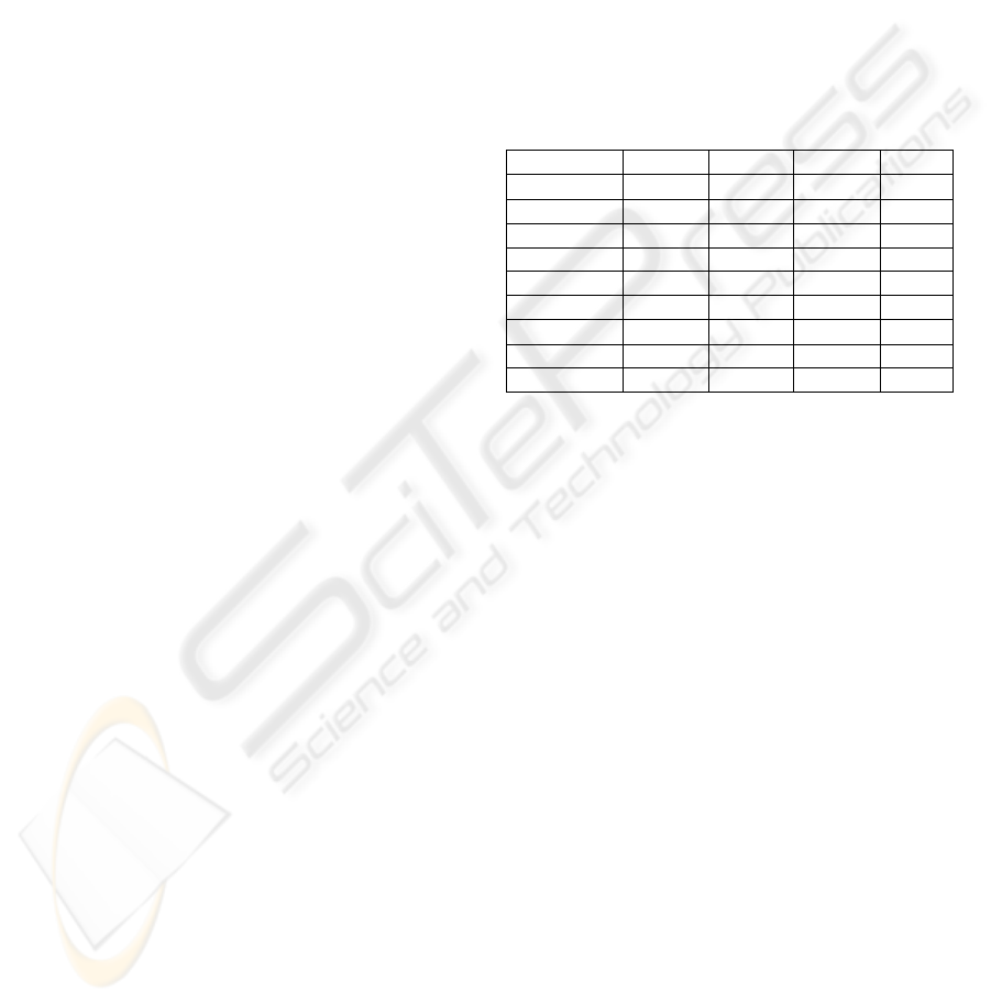
Appendix A: Characteristics of the 4R robot.
Joint N° 1 2 3 4
α (rad)
0 0 0 0
d(m) 0 1 1 1
r(m) 0 0 0 0
a(m) 0 0 0 0
M(kg) 5 4 3 2
Izz(kg.m
2
) 1 0.85 0 0
τ(N.m)
25 20 15 5
F
s
(N.m) 0.7 0.2 0.5 0.2
F
v
(N.m.s) 1 0.2 0.5 0.2
ICINCO 2004 - INTELLIGENT CONTROL SYSTEMS AND OPTIMIZATION
128
