
MULTIPLE ORGAN FAILURE DIAGNOSIS USING ADVERSE
EVENTS AND NEURAL NETWORKS
´
Alvaro Silva Paulo Cortez Manuel Santos
Hospital Geral de Santo Ant
´
onio DSI, Universidade do Minho DSI, Universidade do Minho
Porto, Portugal Guimar
˜
aes, Portugal Guimar
˜
aes, Portugal
Lopes Gomes Jos
´
e Neves
Inst. de Ci
ˆ
encias Biom
´
edicas Abel Salazar DI, Universidade do Minho
Porto, Portugal Braga, Portugal
Keywords:
Intensive Care Medicine, Classification, Clinical Data Mining, Multilayer Perceptrons.
Abstract:
In the past years, the Clinical Data Mining arena has suffered a remarkable development, where intelligent
data analysis tools, such as Neural Networks, have been successfully applied in the design of medical systems.
In this work, Neural Networks are applied to the prediction of organ dysfunction in Intensive Care Units. The
novelty of this approach comes from the use of adverse events, which are triggered from four bedside alarms,
being achieved an overall predictive accuracy of 70%.
1 INTRODUCTION
Scoring the severity of illness has become a daily rou-
tine practice in Intensive Care Units (ICUs), with sev-
eral metrics available, such as the Acute Physiology
and Chronic Health Evaluation System (APACHE II)
or the Acute Physiology Score (SAPS II), just to name
a few (Teres and Pekow, 2000). Yet, most of these
prognostic models (given by Logistic Regression) are
static, being computed with data collected within the
first 24 hours of a patient’s admission. This will pro-
duce a limited impact in clinical decision making,
since there is a lack of accuracy of the patient’s con-
dition, with no intermediate information being used.
On the other hand, the Clinical Data Mining is a
rapidly growing field, which aims at discovering pat-
terns in large clinical heterogeneous data (Cios and
Moore, 2002). In particular, an increasing attention
has been set of the use of Neural Networks (connec-
tionist models that mimic the human central nervous
system) in Medicine, with the number of publications
growing from two in 1990 to five hundred in 1998
(Dybowski, 2000).
The interest in Data Mining arose due to the rapid
emergence of electronic data management methods,
holding valuable and complex information (Hand
et al., 2001). However, human experts are limited and
may overlook important details, while tecniques such
as Neural networks have the potential to solve some
of these hurdles, due to capabilities such as nonlinear
learning, multi-dimensional mapping and noise toler-
ance (Bishop, 1995).
In ICUs, organ failure diagnosis in real time is a
critical task. Its rapid detection (or even prediction)
may allow physicians to respond quickly with therapy
(or act in a proactive way). Moreover, multiple organ
dysfunction will highly increase the probability of the
patient’s death.
The usual approach to detect organ failure is based
in the Sequential Organ Failure Assessment (SOFA),
a diary index, ranging from 0 to 4, where an organ
is considered to fail when its SOFA score is equal or
higher than 3 (Vincent et al., 1996). However, this
index takes some effort to be obtained (in terms of
time and costs).
This work is motivated by the success of previ-
ous applications of Data Mining techniques in ICUs,
such as predicting hospital mortality (Santos et al.,
2002). The aim is to study the application of Neu-
ral Networks for organ failure prediction (identified
by high SOFA values) of six systems: respiratory, co-
agulation, liver, cardiovascular, central nervous and
renal. Several approaches will be tested, using differ-
ent feature selection, training and modeling configu-
rations. A particular focus will be given to the use of
daily intermediate adverse events, which can be auto-
matically obtained from four hourly bedside measure-
ments, with fewer costs when compared to the SOFA
score.
The paper is organized as follows: first, the ICU
clinical data is presented, being preprocessed and
transformed into a format that enables the classifica-
401
Silva Á., Cortez P., Santos M., Gomes L. and Neves J. (2004).
MULTIPLE ORGAN FAILURE DIAGNOSIS USING ADVERSE EVENTS AND NEURAL NETWORKS.
In Proceedings of the Sixth International Conference on Enterprise Information Systems, pages 401-408
DOI: 10.5220/0002623804010408
Copyright
c
SciTePress
tion task; then, the neural models for organ failure
diagnosis are introduced; next, a description of the
different experiments performed is given, being the
results analyzed and discussed; finally, closing con-
clusions are drawn.
2 MATERIALS AND METHODS
2.1 Clinical Data
In this work, a part of the EURICUS II database
(www.frice.nl) was adopted which contains data
related to 5355 patients from 42 ICUs and 9 Euro-
pean Union countries, collected during a period of 10
months, from 1998 to 1999. The database has one en-
try (or example) per each day (with a total of 30570),
being its main features described in Table 1:
• The first six rows denote the SOFA values (one for
each organ) of the patient’s condition in the previ-
ous day. In terms of notation, these will be denoted
by SOF A
d−1
, where d represents the current day.
• The case mix appears in the next four rows, an in-
formation that remains unchanged during the pa-
tient’s internment, containing: the admission type
(1 - Non scheduled surgery, 2 - Scheduled surgery,
3 - Physician); the admission origin (1 - Surgery
block, 2 - Recovery room, 3 - Emergency room, 4
- Nursing room, 5 - Other ICU, 6 - Other hospi-
tal, 7 - Other sources); the SAPSII score (a mortal-
ity prediction index, where higher values suggest a
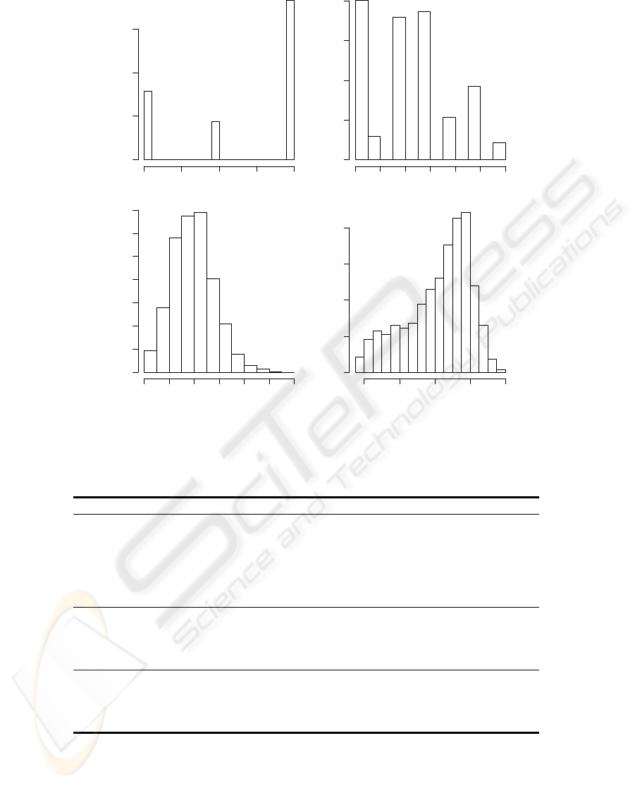
high death probability) and the patient’s age. Fig-
ure 1 shows the frequency distributions of these at-
tributes.
• Finally, the last four rows denote the intermediate
outcomes, which are triggered from four monitored
biometrics: the systolic Blood Pressure (BP); the
Heart Rate (HR); the Oxygen saturation (O2); and
the URine Output (UR). A panel of EURICUS II
experts defined the normal ranges for these four
variables (Tables 2 and 3). Each event (or critical
event) is defined as a binary variable, which will be
set to 0 (false), if the physiologic value lies within
the advised range; or 1 (true) else, according to the
time criterion.
Before attempting modeling, the data was prepro-
cessed, in order to set the desired classification out-
puts. First, six new attributes were created, by slid-
ing the SOF A
d−1
values into each previous exam-
ple, since the intention is to predict the patient’s con-
dition (SOF A
d
) with the available data at day d
(SOF A
d−1
, case mix and adverse events). Then,
the last day of the patient’s admission entries were
discarded (remaining a total of 25309), since in this
cases, no SOF A
d
information is available. Finally,
the new attributes were transformed into binary vari-
ables, according to the expression:
0 , if SOF A
d
< 3 (false, no organ failure)
1 , else (true, organ dysfunction)
(1)
2.2 Neural Networks
In MultiLayer Perceptrons, one of the most popular
Neural Network architectures, neurons are grouped
into layers and only forward connections exist
(Bishop, 1995). Supervised learning is achieved by
an iterative adjustment of the network connection
weights (the training procedure), in order to minimize
an error function, computed over the training exam-
ples (cases).
The state of a neuron (s
i
) is given by (Haykin,
1999):
s
i
= f(w
i,0
+
X
j∈I
w
i,j
× s
j
) (2)
where I represents the set of nodes reaching node
i, f the activation function (possibly of nonlinear
nature), w
i,j
the weight of the connection between
nodes j and i (when j = 0, it is called bias); and
s
1
= x
1
, . . . , s
n
= x
n
, being x
1
, . . . , x
n
the input
vector values for a network with n inputs.
i,0
w
i
i,j
w
j
Hidden Layer
Input Layer
Output Layer
x
x
1
2
x
3
+1
+1
+1
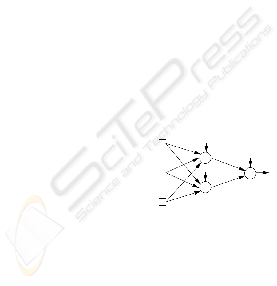
Figure 2: A fully connected network with 3 inputs, 2 hidden
nodes, 1 output and bias connections.
All experiments reported in this work will be con-
ducted using a neural network object oriented pro-
gramming environment, developed in JAVA.
Fully connected Multilayer Perceptrons with bias
connections, one hidden layer (with a fixed num-
ber of hidden nodes) and logistic activation functions
(f(x) =
1
1+e
−x
) were adopted for the organ failure
classification (Figure 2). Only one output node is
used, since each organ system will be modeled by a
different network. This splitting is expected to facili-
tate the Neural Network learning process. Therefore,
ICEIS 2004 - ARTIFICIAL INTELLIGENCE AND DECISION SUPPORT SYSTEMS
402
ADMTYPE
Frequency
1.0 1.5 2.0 2.5 3.0
0 5000 10000 15000
ADMFROM
Frequency
1 2 3 4 5 6 7
0 2000 4000 6000 8000
SAPSII
Frequency
0 20 40 60 80 100 120
0 1000 3000 5000 7000
AGE
Frequency
20 40 60 80 100
0 1000 2000 3000 4000
Figure 1: The case mix histograms.
Table 1: The clinical data attributes.
Attribute Description Domain Values
respirat Respiratory {0, 1, 2, 3, 4}
coagulat Coagulation {0, 1, 2, 3, 4}
liver Liver {0, 1, 2, 3, 4}
cardiova Cardiovascular {0, 1, 2, 3, 4}
cns Central nervous system {0, 1, 2, 3, 4}
renal Renal {0, 1, 2, 3, 4}
admtype Admission type {1, 2, 3}
admfrom Admission origin {1, 2, . . . , 7}
sapsII SAPSII score {0, 1, . . . , 160}
age Patients’ age {18, 19, . . . , 100}
NBP Number of daily BP events and critical events {0, 1, . . . , 28}
NHR Number of daily HR events and critical events {0, 1, . . . , 26}
NO2 Number of daily O2 events and critical events {0, 1, . . . , 30}
NUR Number of daily UR events and critical events {0, 1, . . . , 29}
the predicted class (P
k
) for the k example is given the
nearest class value:
P
k
=
½
0 , if s
k,o
< 0.50
1 , else
(3)
where s
k,o
denotes the output value for the o output
node and the k input example.
Before feeding the Neural Networks, the data
was preprocessed: the input values were standard-
ized into the range [−1, 1] and a 1-of-C encoding
(one binary variable per class) was applied to the
nominal attributes (non ordered) with few categories
MULTIPLE ORGAN FAILURE DIAGNOSIS USING ADVERSE EVENTS AND NEURAL NETWORKS
403

Table 2: The event time ranges.
Event
Suggested Continuously Intermittently
Range Out of Range Out of Range
BP (mmHg) 90 − 180 ≥ 10
0
≥ 10
0
in 30
0
O2 (%) ≥ 90 ≥ 10
0
≥ 10
0
in 30
0
HR (bpm) 60 − 120 ≥ 10
0
≥ 10
0
in 30
0
UR (ml/hour) ≥ 30 ≥ 1 hour
Table 3: The critical event time ranges.
Critical Suggested Continuously Intermittently Event
Event Range Out of Range Out of Range Anytime
BP (mmHg) 90 − 180 ≥ 60
0
≥ 60
0
in 120
0
BP < 60
O2 (%) ≥ 90 ≥ 60
0
≥ 60
0
in 120
0
O2 < 80
HR (bpm) 60 − 120 ≥ 60
0
≥ 60
0
in 120
0
HR < 30 ∨ HR > 180
UR (ml/hour) ≥ 30 ≥ 2 hours ≤ 10
(SOF A
d−1
, admtype and admfrom). For example,
the admtype variable is fed into 3 input nodes, accord-
ing to the scheme:
1 → −1 −1 1
2 → −1 1 −1
3 → −1 −1 1
At the beginning of the training process, the net-
work weights are randomly set within the range [-1,1].
Then, the RPROP algorithm (Riedmiller, 1994) is ap-
plied, due to its faster convergence and stability, be-
ing stopped when the training error slope is approach-
ing zero or after a maximum of E epochs (Prechelt,
1998).
2.2.1 Statistics
To insure statistical significance, 30 runs were applied
in all tests, being the accuracy estimates achieved us-
ing the Holdout method (Flexer, 1996). In each sim-
ulation, the available data is divided into two mutu-
ally exclusive partitions, using stratified sampling: the
training set, used during the modeling phase; and the
test set, being used after training, in order to compute
the accuracy estimates.
A common tool for classification analysis is the
confusion matrix (Kohavi and Provost, 1998), a ma-
trix of size L × L, where L denotes the number of
possible classes (domain). This matrix is created by
matching the predicted (test result) and actual (pa-
tients real condition) values. When L = 2 and there
are four possibilities (Table 4): the number of True
Negative (TN), False Positive (FP), False Negative
(FN) and True Positive (TP) classifications.
From the matrix, three accuracy measures can be
defined (Essex-Sorlie, 1995): the Sensitivity (also
Table 4: The 2 × 2 confusion matrix.
↓ actual \ predicted → negative positive
negative T N F P
positive F N T P
known as recall and Type II Error); the Specificity
(also known as precision and Type I Error); and the
Accuracy, which gives an overall evaluation. These
metrics can be computed using the following equa-
tions:
Sensitivity =
T P
F N+T P
× 100 (%)
Specif icity =
T N
T N+F P
× 100 (%)
Accuracy =
T N+T P
T N+F P +F N +T P
× 100 (%)
(4)
3 RESULTS
3.1 Feature Selection
Four different feature selection configurations will be
tested, in order to evaluate the input attribute impor-
tance:
A - which uses only the SOF A
d−1
values (1 vari-
able).
B - where all available input information is used
(SOF A
d−1
of the corresponding organ system, the
case mix and the adverse events, in a total of 9 at-
tributes);
C - in this case, the SOF A
d−1
is omitted (8 vari-
ables); and
ICEIS 2004 - ARTIFICIAL INTELLIGENCE AND DECISION SUPPORT SYSTEMS
404

D - which uses only the four adverse outcomes.
Since the SOFA score takes costs and time to obtain,
in this study, a special attention will be given to the
last two settings.
In the initial experiments, it was considered more
important to approach feature selection than model
selection. Due to time constrains, the number of hid-
den nodes was set to round(N/2), where N denotes
the number of input nodes (N = 5, N = 21, N = 16
and N = 4, for the A, B, C and D setups, respec-
tively); and round(x) gives nearest integer to the x
value.
The commonly used 2/3 and 1/3 partitions were
adopted for the training and test sets (Flexer, 1996),
while the maximum number of training epochs was
set to E = 100. Each input configuration was tested
for all organ systems, being the accuracy measures
given in terms of the mean of thirty runs (Table 5).
The A selection manages to achieve a high per-
formance, with an Accuracy ranging from 86% to
97%, even surpassing the B configuration. This is
not surprising, since it is a well established fact that
the SOF A is a adequate score for organ dysfunction.
Therefore, the results suggest that there is a high cor-
relation between SOF A
d−1
and SOF A
d
.
When the SOF A index is omitted (C and D), the
Accuracy values only decay slightly. However, this
measure (which is popular within Data Mining com-
munity) is not sufficient in Medicine. Ideally, a test
should report both high Sensitivity and Specificity val-
ues, which suggest a high level of confidence (Essex-
Sorlie, 1995). In fact, there seems to be a trade-
off between these two characteristics, since when the
SOF A values are not present (Table 5), the Sensi-
tivity values suffer a huge loss, while the Specificity
values increase.
3.2 Balanced Training
Why do the A/B selections lead to high Accuracy
/Specificity values and low Sensitivity ones? The an-
swer may be due to the biased nature of the organ
dysfunction distributions; i.e., there is a much higher
number of false (0) than true (1) conditions (Figure
3).
One solution to solve this handicap, is to balance
the training data; i.e., to use an equal number of true
and false learning examples. Therefore, another set
of experiments was devised (Table 6), using random
sampling training sets, which contained 2/3 of the
true examples, plus an equal number of false exam-
ples. The test set was composed of the other 1/3 posi-
tive entries. In order to achieve a fair comparison with
the previous results, the negative test examples were
randomly selected from the remaining ones, with a
distribution identical to the one found in the original
dataset (as given by Figure 3).
The obtained results show a clear improvement in
the Sensitivity values, specially for the C configu-
ration, stressing the importance of the case mix at-
tributes. Yet, the overall results are still far from the
ones given by the A selection.
3.3 Improving Learning
Until now, the main focus was over selecting the cor-
rect training data. Since the obtained results are still
not satisfactory, the attention will move towards bet-
ter Neural Network modeling. This will be achieved
by changing two parameters: the number of hidden
nodes and the maximum number of training epochs.
Due to computational power restrictions, these factors
were kept fixed in the previous experiments. How-
ever, the adoption of balanced training leads to a con-
siderable reduction of the number of training cases,
thus reducing the required training time.
Several experimental trials were conducted, using
different combinations of hidden nodes (H = 4, 8,
16 and 32) and maximum number of epochs (E =
100, 500 and 1000), being selected the configuration
which gave the lowest training errors (H = 16 and
E = 1000). These setup lead to better results, for all
organ systems and accuracy measures (Table 6).
To evaluate the obtained results, a comparison
with other Machine Learning classifiers was per-
formed (Table 7), using two classical methods from
the WEKA Machine Learning software (Witten and
Frank, 2000): Naive Bayes - a statistical algorithm
based on probability estimation; and JRIP - a learner
based on ”IF-THEN” rules.
Although presenting a better Accuracy, the Naive
Bayes tends to emphasize the Specificity values, giv-
ing poor Sensitivity results. A better behavior is
given by the JRIP method, with similar Sensitivity and
Specificity values. Nevertheless, the Neural Networks
still exhibit the best overall performances.
4 CONCLUSIONS
The surge of novel bio-inspired tools, such as Neural
Networks, has created new exciting possibilities for
the field of Clinical Data Mining. In this work, these
techniques were applied for organ failure diagnosis
of ICU patients.
Preliminary experiments were drawn to test several
feature selection configurations, being the best results
obtained by the solely use of the SOFA value, mea-
sured in the previous day. However, this score takes
much more time and costs to be obtained, when com-
pared with the physiologic adverse events. Therefore,
another set of experiments were conducted, in order
MULTIPLE ORGAN FAILURE DIAGNOSIS USING ADVERSE EVENTS AND NEURAL NETWORKS
405

Table 5: The feature selection performances (in percentage).
Organ
A B C D
Acc. Sen. Spe. Acc. Sen. Spe. Acc. Sen. Spe. Acc. Sen. Spe.
respirat 86.3 72.4 90.2 86.2 70.0 90.8 77.9 4.4 98.8 77.6 1.8 99.4
coagulat 97.4 68.8 98.7 97.3 59.6 99.0 95.8 4.6 99.9 95.7 0.0 100
liver 98.3 68.6 99.1 98.3 60.2 99.4 97.3 7.6 99.9 97.3 0.0 100
cardiova 94.2 84.1 96.3 94.2 84.0 96.3 82.8 7.5 99.0 82.2 0.5 99.8
cns 95.7 92.7 96.4 95.7 92.3 96.4 83.5 23.4 97.1 81.6 0.4 99.9
renal 95.5 71.3 97.8 95.3 66.6 98.1 91.4 5.7 99.7 91.1 0.3 100
Mean 94.6 76.3 96.4 94.5 72.1 96.7 88.1 8.9 99.1 87.6 0.5 99.96
Acc. - Accuracy, Sen. - Sensitivity, Spe - Specificity.
Table 6: The balanced C, D and C improved performances (in percentage).
Organ
C D C (improved)
Acc. Sen. Spe. Acc. Sen. Spe. Acc. Sen. Spe.
respirat 61.3 66.4 59.8 67.1 41.1 74.5 63.3 70.4 61.3
coagulat 67.6 66.8 67.7 73.7 41.5 75.1 70.0 72.0 69.9
liver 70.0 71.6 70.0 66.9 36.5 67.8 72.5 77.3 72.4
cardiova 65.9 62.5 66.7 68.2 37.9 74.8 69.1 66.3 69.8
cns 73.6 63.9 75.7 66.8 36.3 73.7 75.2 72.2 75.8
renal 67.8 65.6 68.0 73.2 37.6 76.6 71.9 70.5 72.0
Mean 67.7 66.2 68.0 69.3 38.5 73.8 70.3 71.5 70.2
Acc. - Accuracy, Sen. - Sensitivity, Spe - Specificity.
Table 7: The classifiers performances for the C selection balanced data (in percentage).
Organ
Naive Bayes JRIP Neural Networks
Acc. Sen. Spe. Acc. Sen. Spe. Acc. Sen. Spe.
respirat 73.5 25.2 87.3 62.8 61.9 63.0 63.3 70.4 61.3
coagulat 83.3 24.8 85.8 67.8 62.4 68.0 70.0 72.0 69.9
liver 70.8 54.3 71.2 75.7 73.7 75.7 72.5 77.3 72.4
cardiova 73.4 33.4 82.0 66.6 70.3 65.8 69.1 66.3 69.8
cns 76.3 41.3 84.2 77.6 74.4 78.3 75.2 72.2 75.8
renal 76.8 45.6 79.9 69.1 68.5 69.2 71.9 70.5 72.0
Mean 75.7 37.4 81.7 69.9 68.5 70.15 70.3 71.5 70.2
Acc. - Accuracy, Sen. - Sensitivity, Spe - Specificity.
ICEIS 2004 - ARTIFICIAL INTELLIGENCE AND DECISION SUPPORT SYSTEMS
406

5000 10000 15000 20000 25000 0
respirat
coagulat
liver
cardinova
cns
renal
Figure 3: The organ failure true (in black) and false (in white) proportions.
to improve the use of the latter outcomes. First, the
training sets were balanced to contain similar propor-
tions of positive and negative examples. Then, the
number of hidden nodes and training epochs was in-
creased. As the result of these changes, an improved
performance was gained, specially in terms of sensi-
tivity.
A final comparison between the SOFA score and
the proposed solution (the C improved setup), still fa-
vors the former, although the Sensitivity values are
close (being even higher for the C configuration in
the coagulation and liver systems). Nevertheless, it
is important to stress the main goal of this work: to
show that is it possible to diagnose organ failure by
using cheap and fast intermediate outcomes (within
our knowledge this is done for the first time). The re-
sults so far obtained give an overall accuracy of 70%,
which although not authoritative, still back this claim.
In addiction, the proposed approach opens room for
the development of automatic tools for clinical de-
cision support, which are expected to enhance the
physician response.
In future research it is intend to improve the perfor-
mances, by exploring different Neural Network types,
such as Radial Basis Functions (Bishop, 1995). An-
other interesting direction is based in the use of alter-
native Neural Network training algorithms, which can
optimize other learning functions (e.g., Evolutionary
Algorithms (Rocha et al., 2003)), since the gradient-
based methods (e.g., the RPROP (Riedmiller, 1994))
work by minimizing the Sum Squared Error, a target
which does not necessarily correspond to maximiz-
ing the Sensitivity and Specificity rates. Finally, it is
intended to enlarge the experiments to other ICU ap-
plications (e.g., predicting life expectancy).
REFERENCES
Bishop, C. (1995). Neural Networks for Pattern Recogni-
tion. Oxford University Press.
Cios, K. and Moore, G. (2002). Uniqueness of Medical
Data Mining. Artificial Intelligence in Medicine, 26(1-
2):1–24.
Dybowski, R. (2000). Neural Computation in Medicine:
Perspectives and Prospects. In et al., H. M., editor,
Proceedings of the ANNIMAB-1 Conference (Artifi-
cial Neural Networks in Medicine and Biology), pages
26–36. Springer.
Essex-Sorlie, D. (1995). Medical Biostatistics & Epi-
demiology: Examination & Board Review. McGraw-
Hill/Appleton & Lange, International edition.
Flexer, A. (1996). Statistical evaluation of neural net-
works experiments: Minimum requirements and cur-
rent practice. In Proceedings of the 13th European
Meeting on Cybernetics and Systems Research, vol-
ume 2, pages 1005–1008, Vienna, Austria.
MULTIPLE ORGAN FAILURE DIAGNOSIS USING ADVERSE EVENTS AND NEURAL NETWORKS
407

Hand, D., Mannila, H., and Smyth, P. (2001). Principles of
Data Mining. MIT Press, Cambridge, MA.
Haykin, S. (1999). Neural Networks - A Compreensive
Foundation. Prentice-Hall, New Jersey, 2nd edition.
Kohavi, R. and Provost, F. (1998). Glossary of Terms. Ma-
chine Learning, 30(2/3):271–274.
Prechelt, L. (1998). Early Stopping – but when? In: Neural
Networks: Tricks of the trade, Springer Verlag, Hei-
delberg.
Riedmiller, M. (1994). Supervised Learning in Multi-
layer Perceptrons - from Backpropagation to Adaptive
Learning Techniques. Computer Standards and Inter-
faces, 16.
Rocha, M., Cortez, P., and Neves, J. (2003). Evolutionary
Neural Network Learning. In Pires, F. and Abreu, S.,
editors, Progress in Artificial Intelligence, EPIA 2003
Proceedings, LNAI 2902, pages 24–28, Beja, Portu-
gal. Springer.
Santos, M., Neves, J., Abelha, A., Silva, A., and Rua,
F. (2002). Augmented Data Mining Over Clinical
Databases Using Learning Classifier System. In Pro-
ceedings of the 4th Int. Conf. on Enterprise Informa-
tion Systems - ICEIS 2002, pages 512–516, Ciudad
Real, Spain.
Teres, D. and Pekow, P. (2000). Assessment data elements
in a severity scoring system (Editorial). Intensive Care
Med, 26:263–264.
Vincent, J., Moreno, R., Takala, J., Willatss, S., Mendonca,
A. D., Bruining, H., Reinhart, C., Suter, P., and Thijs,
L. (1996). The SOFA (Sepsis-related Organ Fail-
ure Assessment) score to describe organ dysfunction
/ failure. Intensive Care Med, 22:707–710.
Witten, I. and Frank, E. (2000). Data Mining: Practi-
cal Machine Learning Tools and Techniques with Java
Implementations. Morgan Kaufmann, San Francisco,
CA.
ICEIS 2004 - ARTIFICIAL INTELLIGENCE AND DECISION SUPPORT SYSTEMS
408
