
Mining Self-similarity in Time Series
Song Meina, Zhan Xiaosu, Song Junde
Beijing University of Posts and Telecommunications,
Xitucheng Road,Beijing, China
Abstract. Self-similarity can successfully characterize and forecast intricate,
non-periodic and chaos time series avoiding the limitation of traditional
methods on LRD (Long-Range Dependence). The potential principals will be
found and the future unknown time series will be forecasted through foregoing
training. Therefore it is important to mine the LRD by self-similarity analysis.
In this paper, mining self-similarity of time series is introduced. And the
practical value can be found from two cases study respectively for season-
variable trend forecast and network traffic.
1 Introduction
The time series is a series of observation data according to time-based sequence
whose value changes with time. The time result is recorded by fixed time interval
which is an important characteristic of time series. It is widely applied in real life for
time series such as the price fluctuation in specified period for stock market, the
arrival time of network service, the birth-rate number for population every year etc.
Time series analysis is that random data series variable with time is analyzed
through probability and statistic methods [1]. Following the continuity principle of all
objects, the future development trend is speculated by statistic analysis based on
history data. This means the following two things. One is that no sudden or jump
movement occurred but progressing with relative short steps. The other is the past and
current phenomena potentially imply the evolution tendency for the future. Therefore
in normal circumstance, the valid result will be achieved for short-term forecast from
time series analysis. To extend into further future there is great limitation for long-
term forecast.
In order to analyze data of time series, the visual inspection tools are used to
record data value and distinguish the characteristics and behaviours of certain
phenomena. For example, to study the increase or decrease direction of the data, the
specific pattern changed with seasons, the related progress should be generated from
proper mathematics model and the forecast analysis is made based on the produced
data.
There are many traditional model for time series analysis, such as ARMA (Auto-
Regression Moving Average) and ARIMA (Auto-Regression Integrated with Moving
Averages). ARMA is a linear model for stationary time series analysis and ARIMA is
widely used for non-stationary series. The common characteristics of the two models
are that the LRD between the values for large time intervals can’t be represented.
Meina S., Xiaosu Z. and Junde S. (2006).
Mining Self-similarity in Time Series.
In Proceedings of the 3rd International Workshop on Computer Supported Activity Coordination, pages 131-136
DOI: 10.5220/0002497501310136
Copyright
c
SciTePress
However the LRD characteristics can’t be neglected. Because the time series
attributes will be changed with cumulative effects[2].
Self-similarity can successfully characterize and forecast intricate, non-periodic
and chaos time series avoiding the limitation of traditional time series analysis on
LRD. The potential principals will be found and the future unknown time series will
be forecasted through foregoing training. Therefore it is important for us to mine the
LRD by self-similarity analysis.
2 Self-similarity in Time Series [3]
If one time series meets the following equation (1), then it is self-similar.
() ( )
d
t
yt a y
a
α
≡
(1)
Here
d
≡ suggests that both sides of this equation from the statistical sense are
completely identical. That is to say, after the following transformation,
1)on the X axis, t→t/a
2)on the Y axis,
the distribution function of a self-similar process named y(t) which carried
parameter α still remains unchanged. In this equation the exponent α is called self-
yay
α
→
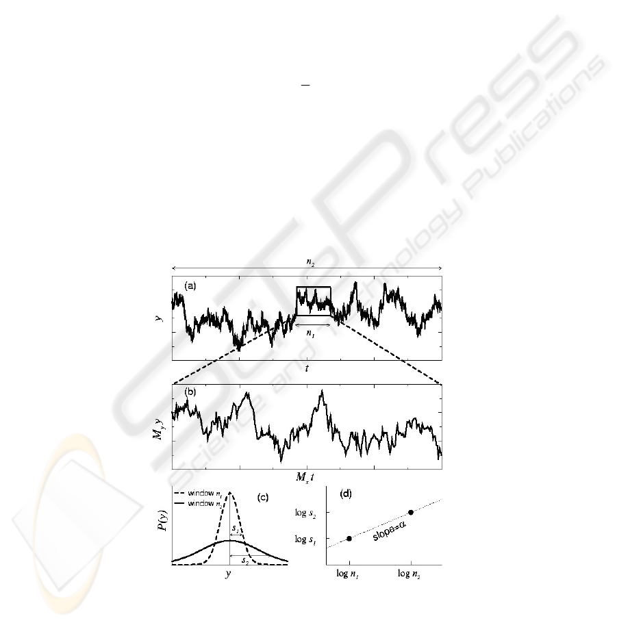
Fig. 1. Self-similarity of a time series.
132

similarity parameter.
However, in fact it is almost impossible to judge whether the two processes
mentioned above are completely identical or not. Because the strict standard requests
that the two processes possess the completely same distribution function, which
means not only the arithmetic mean and variance, but also all the higher order
moments are identical. Thus a relative weakened standard is usually adopted to make
an approximately approached judgment to above equality. That is just checking
whether the average mean and variance, such as first moment and second moment, of
the equation (1) are equal or not.
Fig.1 shows the self-similarity of time series.
(a) A time series with self-similar is shown on the two windows with different
time-scale n
1
and n
2
.
(b) Amplify the smaller window with time-scale n
2
according to time-scales n
1
.
Let’s pay an attention to the two figures in (a) and (b).When the different amplified
multiple M
x
and M
y
are adopted respectively in X axis and Y axis, the fluctuation
curves are so close.
(c) In the possible distribution function P(y) for the two variables y
respectively from windows in (a). Here s
1
and s
2
shows the standard deviation of the
two distribution functions respectively.
(d) The log-log relationship between s and n which is the window size.
The parameter α in equation (1) needs to be abstracted from a given time series.
And the following is the calculation formula.
α=lnM
y
/
ln M
x
(2)
The following equation (3) will be created when put the two parameters M
x
=n
2
/n
1
,
M
y
=s
2
/s
1
into the corresponding position in the equation (2)
(3)
In order to analyze the self-similarity characteristic of given time series, the
following steps should be done.
1) Divide any given observation window into many same size and independent
subsets. To achieve the more reliable value, the average of s in the all subsets
should be calculated.
2) Repeat the above process continually. Then draw these s-n couples on the log-
log plot to estimate the self-similarity parameter α.
The method described above can be no more than applied to certain non-
stationary time series, especially to these with slow movement trend. This means not
all non-stable time series can be well handled with this method. Concerning the self-
similarity parameter, which is also named the Hurst parameter, of most of non-
stationary time series can be precisely estimated through Whittle Estimator method,
which is the practical application of maximal possibility method[4][5]. Whittle
Estimator can provide the confidence interval of the Hurst parameter.
Take the FGN (fractional Gaussian Noise) for example to show the application
of Whittle Estimator in the Hurst parameter estimation. If the data derive from the
FGN procession, the estimated value of Hurst can be gained through minimizing the
value of function Q (H). In the following equation (4), the H is equal to α
mentioned above.
12
12
lnln
lnln
ln
ln
nn
ss
M
M
x
y
−
−
==
α
133

(4)
Therein
)(
ω
NI
is the estimated value of a spectral density got out through
Fourier series transformation on time period N, which is defined in the discrete time {
X
t
, t=0,1,2,3……}by a random process X(t).
(5)
),( HS
ω
in (6) is the spectral density.
S(ω,H
)≈
C
f
|ω|
1-2H
,
ω → 0
(6)
The estimated value of C
f
is shown in (7).
∑
=
−
=
N
j
j
jN
f
H
I
N
C
1
21
)(1
ω
ω
(7)
So for the discrete state, equation (8) comes into existence.
)log(
1
)(
21
)(
1
21
)(
)(
H
jHf
N
j
H
jHf
jN
C
C
I
N
HQ
−
=
−
+=
∑
ω
ω
ω
(8)
An equation (9) will be built by putting the value of function (7) into the right
location in function (8).
∑
∑
=
=
−
−
++=
N
j
j
N
j
H
j
jN
N
H
I
N
N
HQ
1
1
21
)log(
1
)21(
)
)(
1
log(1)(
ω
ω
ω
(9)
Therein the value of ω
j
can be 2π/N,4π/N,…, 2π.
In this way, the value of Hurst parameter can be estimated through minimizing
the value of equation (9).
3 Self-similarity Applied in Data Mining
The data mining of time series, specifically, implies that the useful information can be
got in the database composed of time-based sequence or event whose value changes
with time. It includes trend analysis, similarity query, mining of sequential patterns
and periodic-mode mining [6].
3.1 Self-similarity Applied in Trend Analysis
The long-term trend change of time-based sequence reflects a kind of trend curve
during a relative longer time interval. Given a group of fixed data{x
t
, t=0,1,2
,
…}, the
ωωω
ω
ω
π
π
π
π
dHSd
HS
I
HQ
N
∫∫
−−
+= ),(
),(
)(
)(
2
1
2
1
)(
∑
=
=
N
k
ik
kN
ex
N
I
ω
π
ω
134

normal methods deciding sequence trend can be used to calculate n-order moving
average according to the following arithmetic mean equation sequence.
(10)
Smoothness of time series by moving average can decrease the abnormal
fluctuation, which deviates from the original sequence. After that, in equation (10),
the right n-order weighted average made by adopting weighted average can reduce the
influence of the extreme data on sequential trend of the whole time series. The trend
curve can also be got though curve fitting by least square method.
Both methods mentioned above can not find the LRD characteristic. The time
series, whose value changes with seasons, is the typical ones with long-range
dependency. The season-variable time series indicates that there is an identical or
almost identical mode which appears repeatedly in the special months of the several
consecutive years. For example, dramatic traffic increasing during Spring Festival is
an almost identical mode for statistical data based on every year. Long-range
dependency is an inherent attribute for self-similarity. In order to analyze the long-
range dependency trend, self-similarity method should be introduced. In general, the
season-variable time series forecast methods can be described as followings.
3) Based on the self-similarity analysis on time series from the previous years, the
Hurst parameter will be created. And consequently the principal trend for the
whole time series can be built.
4) Combined with the traffic increasing of current recorded year, let’s just make the
corresponding amplitude shift. Then the rough trend curve will be presented with
season change.
Thus traffic forecast analysis will be made for long-term traffic.
3.2 Self-similarity Applied in Mining Network Traffic
Self-similarity is an important character of web traffic [7]. That means it is always
possible for the larger peak period occurs. In order to mine the behaviour pattern on
different time scales, traditional methods can’t capture the most distinct
characteristics of the web traffic. Therefore self-similarity analysis must be made to
mine the recorded time series on different time scales.
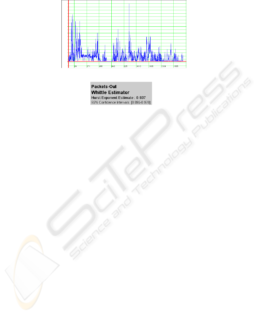
Figure 2 is the collected data from China Mobile, which represent the number of
packets outputting from VPN (Virtual Private Networks) gateway every 5 minutes
during work-hours. A tool for self-similarity and LRD analysis is designed in [8] and
the Hurst parameter is 0.937 with 95% confidence intervals, which is shown in Figure
3.
From Figure 3, we can observe that the VPN gateway is provided with self-
similarity arrival. So no classical queuing theory can be applied to evaluation the
system performance. For they all suppose the Poisson arrival. This will avoid the
optimal performance estimation of the studied systems.
"
"
""
,
,,
132
21110
n
xxx
n
xxx
n
xxx
n
nn
+
−
+++
+
+
++
+
+
135
4 Conclusions and the Future Works
The traditional methods can get the valid results for short-term forecast from time
series analysis. To extend into further future there is great limitation for long-term
forecast. In this paper, how to do self-similarity analysis on time series is introduced.
Suggestions on applying self-similarity into data mining are put forward. From the
mentioned two cases, both how to forecast time series changed with seasons and how
to mine the behaviour patterns on different time scales are discussed. The detailed
implementation will be studied in the further research.
References
1. G.E.P Box and G.M.Jenkins, 1976. Time Series analysis: forecasting and control. 2nd
Edition, Holden_Day, San Francisco.
2. Feder J, 1988. Fractals. New York: Plenum Press.
3. Beran J, 1994. Statistics for Long-Memory Processes. New York: Chapman & Hall.
4. S. Molnár, T. D. Dang, A. Vidács, 1999. Heavy-Tailedness, Long-Range Dependence and
Self-similarity in Data Traffic. 7th International Conference on Telecommunication
Systems Modeling and Analysis, Nashville, Tennessee, USA.
5. Lin Chuang
, 2001. Performance Analysis on Computer Networks and Computer
Systems.Tsing Hua Press.
6. Jiawei Han,Micheline Kamber, 2001. Data Ming: Concepts and Technoloties. China
Machine Press.
7. M.Crovella, A.Bestavros, 1997. Self-similarity in World Wide Web Traffic: Evidence and
Possible Causes.IEEE/ACM Transactions on Networking,5(6):835-846.
8. Thomas Karagiannis, Michalis Faloutsos, 2005. The SELFIS Tool.
http://www.cs.ucr.edu/~tkarag/Selfis/Selfis.html
2500
5500
7500
10000
12500
Fig. 2. Packet Number of the VPN Gateway
Fig. 3. Hurst Parameter
136
