
COINCIDENCE BASED MAPPING EXTRACTION WITH GENETIC
ALGORITHMS
Vahed Qazvinian, Hassan Abolhassani and S. Hossein Haeri
Web Intelligence Lab, Computer Engineering Department
Sharif University of Technology, Tehran, Iran
Keywords:
Ontology Matching, Ontology Aligning, Coincidence Based Matching, Alignment Extraction, Genetic Algo-
rithm.
Abstract:
Ontology Aligning is an answer to the problem of handling heterogenous information on different domains.
After application of some measures, one reaches a set of similarity values. The final goal is to extract map-
pings. Our contribution is to introduce a new genetic algorithm (GA) based extraction method. The GA,
employs a structured based weighting model, named “coincidence based model”, as its fitness function. In the
first part of the paper, some preliminaries and notations are given and then we introduce the coincidence based
weighting. In the second part the paper discusses the details of the devised GA with the evaluation results for
a sample dataset.
1 INTRODUCTION
Semantic web is made up of distributed information
that has resulted in designing ontologies to lessen the
heterogeneity. Yet another problem exists: ontologies
themselves may cause heterogeneity. This is when
two ontologies are trying to express same knowledge
or concepts but they use different languages or words
(Euzenat and Valtchev, 2004). This has led to the
problem of ontology aligning.
Ontology aligning has been discussed for a while, to
enable a mapping of two heterogenous information in
different domains. This will make agents which are
using different ontologies, establish interpretability.
This alignment will give a correspondence between
concepts and semantics of two ontologies.
To do an alignment it is customary to first apply some
measures (simple or complex) to reach to some initial
guesses. Then the problem is how to form an ideal
mapping. This problem which is referred to as Map-
ping Extraction is the target of this paper.
After having an explanation of related works in sec-
tion 2, section three shows some definitions and nota-
tions used in the paper. Then section 4 discusses our
coincidence based theory which is the basis for our
GA algorithm discussed in section 5. Section 6 ex-
plains evaluations done on the algorithm and finally
section seven concludes the paper.
2 RELATED WORKS
Unfortunately works on ontology extractions are not
so many, as stated in (Bouquet et al., 2004). In
(Melnik et al., 2002), to extract a reasonable extrac-
tion, Stable Marriage (Gibbons, 1985) problem is dis-
cussed. There are some other approaches, e.g. a ma-
chine learning approach to the problem is discussed in
(Doan et al., 2003), and (Mitra et al., 2003) describe
a probabilistic based model. Some methods tend to a
trade off of different features such as efficiency and
quality, as in QOM (Ehrig and Staab, 2003) and some
have used approaches to integrate various similarity
methods (Ehrig and Sure, 2004).
(Kalfoglou and Schorlemmer, 2003) have come with
a comprehensive review and presentations on the
methods and approaches and the state of art in on-
tology aligning .
According to (Haeri et al., 2006): “no [much] work
is so far done on the problem of Ontology Align-
ment or Ontology Matching in which graph theoretic
backbone of problem is scrutinized.”. With the use
176
Qazvinian V., Abolhassani H. and Hossein Haeri S. (2007).
COINCIDENCE BASED MAPPING EXTRACTION WITH GENETIC ALGORITHMS.
In Proceedings of the Third International Conference on Web Information Systems and Technologies - Web Interfaces and Applications, pages 176-183
DOI: 10.5220/0001271901760183
Copyright
c
SciTePress
of graph theory and such a modeling we believe that
there is a vast area for new work on the problem of
ontology aligning.
3 DEFINITIONS
In this section we will define the notations that are
used throughout the paper. We will start by defining
necessary mathematical backgrounds.
A graph G
i
, by definition, consists of two sets:
V(G
i
),E(G
i
), where V(G
i
) is the set of vertices, and
E(G
i
) is the set of edges. The size of a graph is
|V(G
i
)|, which is denoted by |G|. Lets assume that la-
bels assigned to nodes are chosen from a finite alpha-
bet Σ. Let λ /∈ Σ be a null character, and Σ
λ
= Σ∪ λ.
3.1 Typed Graph
An ontology O
i
, in this paper, is considered as a typed
graph G
i
. A typed graph, as defined in (Haeri et al.,
2006), is denoted by G
i
(V,E,T), where E is of type:
E : V × V → T. labels in T are from Σ
λ
. In such
a graph an edge e between two vertices v
i
j
,v
i
k
with
type t is denoted by: e(v
i
j
,v
i
k
) : t.
In this paper each ontology O
i
is modeled using a
typed graph G
i
where concepts in O
i
are nodes of G
i
and relations and properties of O
i
are typed edges of
the graph.
3.2 Distance
The distance of two concepts belonging to two
different graphs is described as the distance of
their labels in a metric space. Usually this met-
ric distance is described by a distance function,
δ : (Σ
λ
× Σ
λ
)\(λ,λ) → R. So the distance of two
nodes v
i
,v
j
is denoted by δ(label(v
i
),label(v
j
)). For
simplicity we will show it by δ(v
i
,v
j
). This metric
distance, δ, for any v
1
,v
2
,v
3
∈ Σ
λ
should have the
following properties (Haeri et al., 2006):
1. δ(v
1
,v
2
) ≥ 0,δ(v
1
,v
1
) = 0
2. δ(v
1
,v
2
) = δ(v
2
,v
1
) Symmetry
3. δ(v
1
,v
2
) + δ(v
2
,v
3
) ≥ δ(v
1
,v
3
) Transitivity
This distance function can either be a String-Based
distance or any other possible one. In this research,
the distance of two vertices v
i
,v
j
, say δ(v
i
,v
j
), is con-
sidered to be the Levenshtein Distance (Levenshtein,
1966) of their labels.
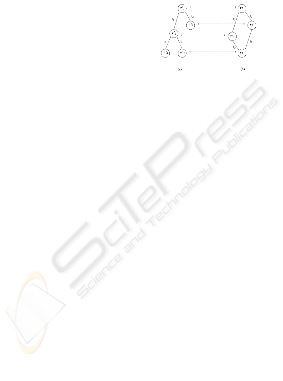
Figure 1: A sample matching of two graphs G
′
,G.
3.3 Ontology Alignment
In this section we will discuss our own understanding
of a one to one matching between ontologies.
A one to one matching
1
of two ontologies O
i
1
,O
i
2
is denoted by m : O
i
1
→ O
i
2
and is a one to one
correspondence between nodes of the two graphs of
O
i
1
,O
i
2
: (G
i
1
, G
i
2
).
(Ehrig and Sure, 2004) define the mapping function
the following way:
• m : O
i
1
→ O
i
2
• ∀v ∈ G
i
1
: m(v) = v
′
if v
′
∈ G
i
2
and δ(v,v
′
) <
t, for t being a threshold
v
′
is the corresponding node of v under the mapping
m. It is clear that with this definition, correspondence
of edges, is determined by the correspondence of
nodes:
∀e(v
1
j
,v
1
k
) : t ∈ E(G
i
1
) : if m(v
1
j
) = v
2
j
6=
/
0,m(v
1
k
) = v
2
k
6=
/
0,and e(v
2
j
,v
2
k
) : t ∈
E(G
i
2
) then m(e(v
1
j
,v
1
k
)) = e(v
2
j
,v
2
k
)
Figure 1 illustrates a sample alignment for two
sample ontologies G
′
,G.
3.4 Edge Preservation
We will call an edge e(v
1
j
,v
1
k
) : t ∈ E(G
i
1
) is pre-
served under the matching m, iff there is an edge
e(m(v
1
j
),m(v
1
k
)) : t ∈ E(G
i
2
). In other words an
edge, e is preserved under matching m if and only if
∃e
′
: e
′
= (m(v
1
j
),m(v
1
k
)),m(e) = e
′
, and is not pre-
served otherwise
The preservation of edges between corresponding
nodes is the key point to find an ideal matching. In
fact in an ideal alignment most of the edges of one
ontology are preserved in the second one.
1
We will sometimes call it Alignment or mapping of two
ontologies
COINCIDENCE BASED MAPPING EXTRACTION WITH GENETIC ALGORITHMS
177

4 COINCIDENCE BASED
WEIGHTING
In this section we introduce and discuss a new weight-
ing model for an alignment, with which we will later
design our genetic algorithm. The coincidence based
alignment weight function is sufficiently discussed in
(Haeri et al., 2006), and here, we will have a brief in-
troduction to it. Before talking about the weight itself,
lets take some time, and discuss the matter.
Consider a mapping m, between two ontologies with
graphs G
i
1
,G
i
2
, and also consider two nodes v
1
j
,v
1
k
∈
V(G
i
1
) and their matches m(v
1
j
),m(v
1
k
). The weight-
ing system should result a high weight if v
1
j
is
close to m(v
1
j
) and also is v
1
k
to m(v
1
k
) and be-
sides, e = (v
1
j
,v
1
k
) : t ∈ E(G
i
1
) is preserved under
m. In this case v
1
j
,v
1
k
are close to m(v
1
j
),m(v
1
k
), and
there is an edge both between v
1
j
,v
1
k
, and between
m(v
1
j
),m(v
1
k
). This case is considered to be the most
desired one and should be given the highest value.
In the second case lets suppose the edge is not pre-
served. Here, a negligible negative point should be
given. The reason for negative point is the fact that,
the edge is not preserved and the structural matching
of the graphs is interrupted. In this case the nodes are
very close but the edge is missing.
The farther any of the nodes is, from its match, the
lower should be the positive value of the matching.
If the edge is preserved, we give this matching a low
positive value. But when the edge is not preserved, in
fact it is an undesired matching. So we give it a nega-
tive point. In this case not only the nodes are far from
their matches, but also the edge is not preserved.
According to above considerations there should be six
different categories: (Suppose G,G
′
are graphs of two
ontologies O,O
′
to be aligned. a, b are concepts from
G, and a
′
,b
′
from G
′
)
• Category I. a and a
′
are too close
2
, and b, b
′
are
close as well. That means, the distance between a,
a
′
is low, and so is the distance between b,b
′
. The
edge between a,b is preserved so this category is
of much importance. This is because actually the
two edges coincide too much.
• Category II. In this category the edge is pre-
served but only one of the a or b is close to its
match. This is good but not as much as the previ-
ous category.
• Category III. The two peers of an edge are
close to their matches, that means, a is close to a
′
and b is close to b
′
. But the edge is not preserved.
This category should not be penalized much, be-
2
in terms of a distance function described before
cause at least concepts are close to their matches
and vertices coincide.
• Category IV. The edge between a,b is not pre-
served, and b if far from b
′
. The only positive
point of such a matching is the fact that a and a
′
are close.
• Category V. and VI. in these categories, both
a,a
′
and b,b
′
are far from one another, and the
difference is in the preservation of edges. Both
cases are not desired and should obtain low points.
According to the above sort and discussions, the
following weigh function is suggested:
w(m) = w
0
(m) − w
l
(m) − w
r
(m)
w
0
(m) =
∑
(v
1
,v
2
):t∈E(G) , (m(v
1
),m(v
2
)):t∈E(G
′
)
f(v
1
)+ f (v
2
)
w
l
(m) =
∑
(v
1
,v
2
):t∈E(G) , (m(v
1
),m(v
2
)):t/∈E(G
′
)
g(v
1
)+g(v
2
)
w
r
(m) =
∑
(v
1
,v
2
):t/∈E(G) , (m(v
1
),m(v
2
)):t∈E(G
′
)
g(v
1
)+g(v
2
)
The functions f and g, referred to as Normaliza-
tion Functions, are in the form:
f : R → R
+
g : R → R
+
f,g are related to the distance function. In fact,
f should be a positive decreasing function, so that
if δ(v,m(v)) grows, it decreases to reduce the pos-
itive point. And on the other hand g should be a
positive increasing function to grow with the growth
of δ(v, m(v)) to increase the negative point for that
match. Normalization functions are defined by tun-
ing the system. This will be described again later.
5 GENETIC ALGORITHM
This section describes the designed genetic algorithm.
Matching two general graphs in polynomial running
time algorithms is impossible, because the problem
in its general case is MAX SNP-Hard (Arora et al.,
1992). So a random search algorithm could be a good
idea when designed carefully. This led us to the idea
of using genetic algorithm.
WEBIST 2007 - International Conference on Web Information Systems and Technologies
178

5.1 Coding a Matching
To code a matching we used hashmaps (Cormen
et al., 2001) in which keys are concepts of one
ontology and entries are concepts of another. Entry
for each key is actually the corresponding node of
that key in the mapping
5.1.1 Pairs
According to the coincidence-based model, we de-
fined Pair, as two concepts from one ontology,
between which there is a relation (So there is
an edge in the graph of that ontology). Fig-
ure 1 shows the alignment of two ontologies.
(v
1
,v
2
),(v
1
,v
3
),(v
3
,v
4
),(v
2
,v
4
) are pairs of G. A pair
also has a weight according to the alignment it in-
volves in.
Clearly speaking, a pair is a function of the form:
P : V ×V × T −→ R
where V is the set of vertices in ontology graph G and
T is a set of labels in Σ
λ
. So an ontology in a match-
ing has a limited number of pairs.
The weight of a pair depends on the alignment in
which the ontology is involved. Let G
i
1
,G
i
2
be two
graphs of two aligned ontology, and v
1
j
,v
1
k
∈ V(G
i
1
).
Also assume an edge between v
1
j
,v
1
k
to be of type t,
e
1
jk
= e(v
1
j
,v
1
k
) : t.
P(v
1
j
,v
1
k
,t) in the alignment of two ontologies is
given by:
P(v
1
j
,v
1
k
,t) =
f(v
1
j
) + f (v
1
k
) e
1
jk
preserved
−(g(v
1
j
) + g(v
1
k
)) e
1
jk
not preserved
−∞ if e
1
jk
/∈ E(G
i
1
)
For the couple of concepts which do not form a pair
the value of P function is set to be −∞. Definition
of pairs, seemed necessary for further crossover
function which will try to improve the structural
matching.
In the alignment of two ontologies, O
i
1
(G
i
1
) ,
O
i
2
(G
i
2
), say m : O
i
1
→ O
i
2
, we also define the
weight of a single concept from one ontology,
W(v
1
j
) where v
1
j
∈ V(G
i
1
), as follows:
if v
1
j
∈ V(G
i
1
),m(v
1
j
) ∈ V(G
i
2
)
W(v
1
j
) =
∑
∀v∈G
i
1
:e(v
1
j
,v):t∈E(G
i
1
)
P(v
1
j
,v,t)
5.1.2 An Example
To make things clear about the definition of pair and
its corresponding weights described above, we give
an example on how to compute these weights.
In the Figure 1 we have:
P(v
1
,v
2
,t
2
) = f (v
1
) + f (v
2
)
P(v
1
,v
3
,t
1
) = f (v
1
) + f (v
3
)
P(v
3
,v
4
,t
3
) = −g(v
3
) − g(v
4
)
P(v
2
,v
4
,t
4
) = −g(v
2
) − g(v
4
)
P(v
1
,v
4
,t
i
) = P(v
2
,v
3
,t
i
) = −∞
W(v
1
) = ( f(v
1
) + f (v
2
)) + ( f(v
1
) + f (v
3
))
W(v
2
) = ( f(v
2
) + f (v
1
)) − (g(v
2
) + g(v
4
))
W(v
3
) = ( f(v
3
) + f (v
1
)) − (g(v
3
) + g(v
4
))
W(v
4
) = −(g(v
4
) + g(v
3
)) − (g(v
4
) + g(v
2
))
Now, with these definitions, it is the time, to clarify
the steps of the genetic algorithm.
5.2 Initialization
As of any other genetic algorithms, a population is
needed. A population is made up of some individ-
uals each of which is a solution to the problem (an
alignment in this problem). The start population, is
initialized randomly, with an initial size of 1000 in-
dividuals. The ideal matching can be reached more
quickly if the initial individuals, are made on the ba-
sis of the labels of concepts, that is if v
1
j
in G
i
1
and
v
2
j
in G
i
2
have same labels, then let v
1
j
corresponds
to v
2
j
in the initial mapping.
5.3 Selection
In each iteration, we sorted the 1000 individuals ac-
cording to their fitness described in section 4 (coinci-
dence based weight function, and we selected the 500
best individuals as parents of next step. From these
500 individuals, with the use of crossover and muta-
tion functions (as we will see later), 1000 new indi-
viduals are created. These 1000 individuals are sent
to the next iteration.
5.4 Crossover
In the crossover function, single nodes are compared
according to their weight. As we described before the
weight of a single node in an alignment is the sum of
weights of pairs in which, that node is included.
Consider two parents between two ontology graphs
G
i
1
,G
i
2
. To make an offspring from two parents, for
every node in G
i
1
, say v
1
j
, the mapping with larger
W(v
1
j
) is copied to the offspring. if m(v
1
j
) in G
i
2
is already assigned with some other node of G
i
1
,
then v
1
j
is put in a reserved list. At the end of the
COINCIDENCE BASED MAPPING EXTRACTION WITH GENETIC ALGORITHMS
179
complete iteration of nodes in G
i
1
, the nodes in that
reserved list are randomly mapped to the unassigned
nodes of G
i
2
. The random assignment is not done in
the middle of the iteration, to prevent nodes of G
i
2
to
be assigned to some random nodes, where they can
be assigned to better nodes later in the iteration. So
this random assignment is postponed until all nodes
of G
i
1
are examined to map to nodes in G
i
2
.
As an example suppose v
1
m
∈ V(G
i
1
) should map to
v
2
m
∈ V(G
i
2
) and v
2
m
is already mapped by some
node from G
i
1
, so if at the time we assign v
1
m
to
some random node like v
2
n
∈ V(G
i
2
). This will
prevent a possible good mapping of v
1
n
to v
2
n
later
in the iteration, because that will make v
2
n
assigned.
So this random matching is delayed until no more
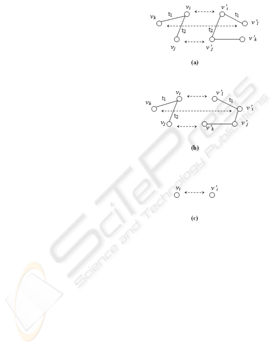
assignment is possible. In Figure 2 two mapping
between two ontologies O,O
′
are shown, and we
want to decide the match node for v
i
∈ V(G) in the
offspring. In parent 1 we have:
W(v
i
) = P(v
i
,v
j
,t
2
)+P(v
i
,v
k
,t
1
) = ( f(v
i
)+ f(v
j
))+
( f(v
i
) + f (v
k
))
and in parent 2 we have:
W(v
i
) = P(v
i
,v
j
,t
2
) + P(v
i
,v
k
,t
1
) = −(g(v
i
) +
g(v
j
)) + ( f(v
i
) + f (v
k
))
f,g are positive functions so amount of W(v
i
) in
parent 1 (Figure 2 (a)) is greater than that of in parent
2 (Figure 2 (b)). So as is seen, the corresponding node
of v
i
∈ V(G) in offspring is chosen by the mapping
shown from parent 1, and therefore is v
′
i
∈ V(G
′
)
This kind of crossover seems reasonable because the
mapping of a single node in the offspring is not worst
than that of the two parents. So by this assumption,
little by little, mappings of nodes will converge to an
ideal ones.
5.5 Mutation
A proportion of the population are mutated with some
probability, different in various situations. In mu-
tation of a mapping of two ontologies with graphs
G
i
1
,G
i
2
, two random nodes from G
i
1
are chosen, and
their matches in G
i
2
are substituted with each other.
Let v
1
j
,v
1
k
∈ V(G
i
1
) are chosen randomly, also let
m(v
1
j
) = v
2
j
∈ V(G
i
2
),m(v
1
k
) = v
2
k
∈ V(G
i
2
). In the
mutation process we just substitute the match nodes
of the selected ones. So the new mapping will be
m(v
1
j
) = v
2
k
∈ V(G
i
2
),m(v
1
k
) = v
2
j
∈ V(G
i
2
).
5.6 Continuation
500 best children from a previous step are sorted de-
creasingly, and form the parents of current step. These
parents produce 1000 new individuals, and the best
500 of these 1000 children are selected as parents
Figure 2: crossover . (a)part of parent 1 matching. (b)part
of parent 2 matching (c) part of offspring.
of next step. The i
th
and i + 1
th
parents involve in
crossover and mutation, and create offsprings. From
the set of all these offsprings and their two parents,
the two best are chosen as children. The last parent
is mixed with the first one to produce last offsprings.
As stated before, after the necessary 1000 children are
made, they are sorted according to the fitness function
and the best 500 are selected for the next step (Figure
3 ).
5.7 End Condition
To end the iteration of GA, we used a threshold for
convergence. The sequential GA continued until the
best mapping among all individuals in the population
WEBIST 2007 - International Conference on Web Information Systems and Technologies
180
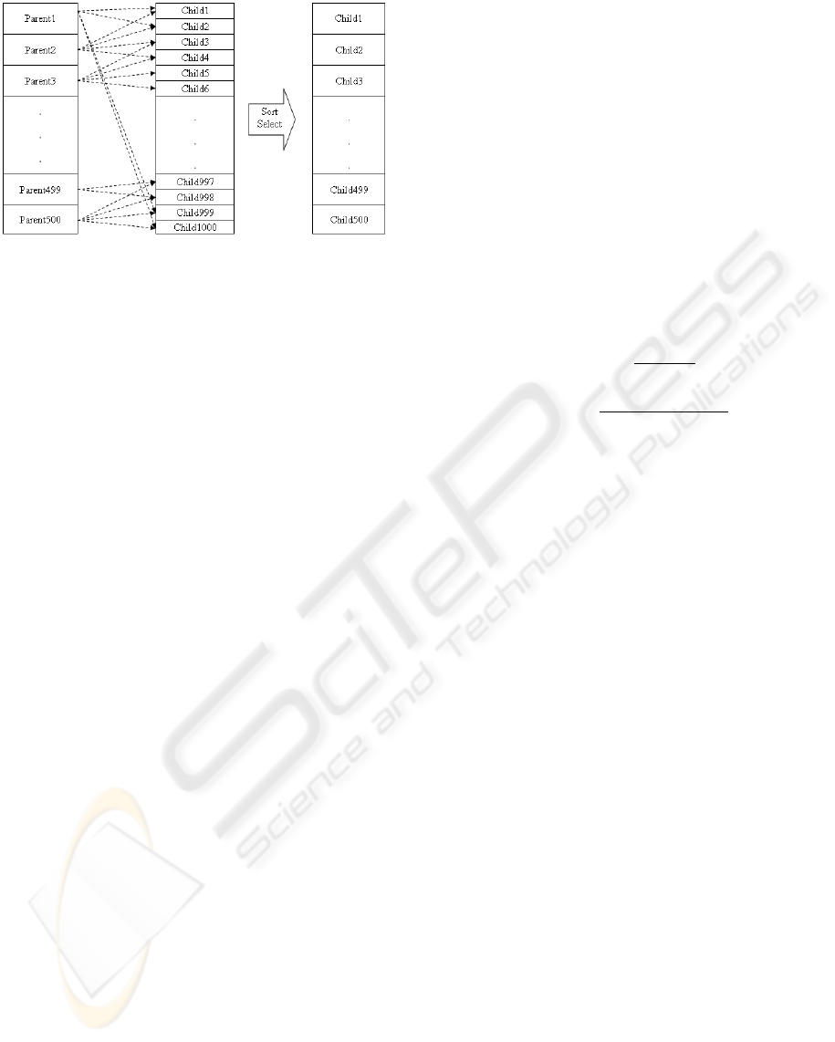
Figure 3: Population generation in each step of GA.
did not improve for more than 15 steps. Such map-
ping is reported as the answer, and the alignment of
two ontologies is then finalized.
6 EVALUATION
To evaluate our Genetic Algorithm, we designed three
kids of experiments. In the first experiment, we tested
the Genetic Algorithm with diverse mutation proba-
bility. In the second experiment, we tried to align to
identical ontologies (actually we aligned one ontol-
ogy with itself). This experiment helped us examine
the efficiency and accuracy of the algorithm, when
two ontologies are more similar to each other. To
verify our contribution, we come with a third experi-
ment, in which we used a naive local search alignment
method.
6.1 Limitations
The coincidence-based ontology matching appears to
be an innovative idea, however there are essential lim-
itations with this method. The most important limita-
tion is the available ontologies and test collections.
Most of them do not have a large taxonomic struc-
ture and so the method does not have enough merit
for them. To test this method we needed large tax-
onomic ontologies. We found “Tourism” ontologies
(tou, ) a suitable test bench with approximately 340
classes and concepts.
6.2 Various Experiments
Characteristics
For the tourism ontologies, an ideal alignment was
given, so that we could have the ideal alignment
of our graphs. The precision measure (Baeza-Yates
and Ribeiro-Neto, 1999) was calculated based on the
given information.
• Experiment 1
As discussed previously, in this experiment we
aligned “TourismA” with “TourismB”. This is
the main experiment of our method, to check
the efficiency of our coincidence-based genetic
algorithm.
In this experiment, from each two parents, we
made one offspring with the use of crossover
function. From the three different individuals
(parents and the offspring) we chose two best of
them, to introduce as children of this amalgama-
tion.
Normalization Functions are as follows:
f(v) =
1
e
δ(v,m(v))
g(v) =
1
e
max(5,15−δ(v,m(v)))
These functions actually satisfy the characteris-
tics expected from f,g (explained in Sec. 4). f
is a decreasing function and decreases with the
growth of δ and g is increasing. Exponential func-
tions were chosen for f,g so that f,g would have
close and comparable values. In fact, these func-
tions match the discussions on positive and neg-
ative points for different categories of a coinci-
dence based weight.
– Experiment 1.1
After the 1000 individuals were created, we
mutated the lower half of the them (with the
mutation function described before) with a
probability of 0.7.
– Experiment 1.2
After the 1000 individuals were created, we
mutated the lower half of the them (with the
mutation function described before) with a
probability of 0.3.
– Experiment 1.3
Mutation was done on each one of the 1000 in-
dividual in the all of the 1000 children with the
probability of 0.5.
• Experiment 2
In this experiment we are aligning “TourismA”
with itself. This actually is a verification that
shows how efficient the genetic algorithm will
work, if two ontologies are more similar and
actually more coincident.
The generation summary is similar to the previous
experiment, and mutation was done on the lower
COINCIDENCE BASED MAPPING EXTRACTION WITH GENETIC ALGORITHMS
181
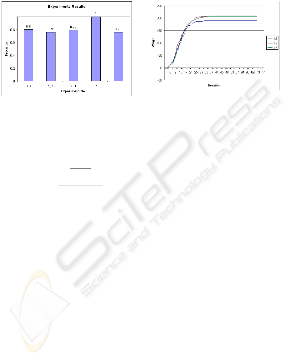
Figure 4: Precision result of experiments.
half of the individuals, with the probability of
0.5.
Normalization Functions are like the previous
experiment,
f(v) =
1
e
δ(v,m(v))
g(v) =
1
e
max(5,15−δ(v,m(v)))
• Experiment 3
This experiment actually provides a baseline com-
parison of the GA method with a naive local
search method. In this part, we implemented
a naive hill-climbing local search method. For
the start point, we made an initial alignment. In
this initial alignment, all concepts in “TourismA”
where matched with concepts in “TourismB”. For
a node v
j
in TourismA if there were a node v
′
j
with
label label(v
j
) in TourismB, we matched v
j
with
v
′
j
. Otherwise we mapped v
j
to a random node of
TourismB.
After that, in each iteration, the best single change
(mutation) was preformed to improve the weight
value of alignment. We iterated the method until
almost 1000 steps, where, the results did not im-
prove for more than 15 steps.
6.3 Results
Figure 4 shows the result of the above experiments in
precision (Baeza-Yates and Ribeiro-Neto, 1999). As
it is shown, with equal graphs Genetic algorithm finds
the best matching and precision is 1.
In our experiments, the distance threshold, which we
talked about in section 3.3, is set to be 4. We chose
this number by experience, however there could be
Figure 5: Convergence of results in GA.
other solutions to determine this number, like ma-
chine learning techniques, etc. The discussion on how
to define this threshold and the distance function, is
beyond the scope of this paper. With other experi-
ments, however, the result is a little inaccurate in com-
parison with the ideal alignment and precision is ap-
proximately 0.8.
We also did an investigation on iteration number and
convergence of the result in this genetic algorithm for
Experiment 1. The results are shown in figure 5 .
7 CONCLUSION AND FUTURE
WORK
Genetic Algorithm seems efficient in the problem
of ontology alignment extraction. It also converge
rapidly, for example after approximately 40 iterations
in our experiments. This number can even be reduced
by choosing a biased initial population, where labels
can be involved to choose better initial mappings.
Coincidence Based approach, when improved and
used as a fitness function of a genetic algorithm might
be useful when ontologies have a more taxonomic
structure. There is also some weakness with genetic
algorithms. One of them is the dependency of results
to initial population. The more important weakness is
when two ontologies are in the form of sparse graphs
or even forests, in that case the domain for crossover
is not a soft one, and small changes in an individual in
crossover or mutation might take it to a very far point,
and most of the time, an out of goal point of course.
Work is now being done on tree ontologies, and rela-
tions in them. Once we can align tree ontologies, we
can model ontologies as trees and align these trees.
We are also interested to extend our theory and mech-
anisms for matching ontologies based on their shapes,
graph areas, etc.
WEBIST 2007 - International Conference on Web Information Systems and Technologies
182

REFERENCES
Tourism ontology FOAM. avail-
able online: http://www.aifb.uni-
karlsruhe.de/WBS/meh/foam/ontologies/.
Arora, A., Lun, C., Motwani, R., Sudan, M., and Szegedy,
M. (1992). Proof verification and hardness of approx-
imation problems. In 33rd IEEE symposium on the
Foundations of Computer Science (FOCS), pages 14–
23.
Baeza-Yates, R. and Ribeiro-Neto, B. (1999). Modern In-
formation Retrieval. Addison Wesley.
Bouquet, P., Euzenat, J., Franconi, E., Serafini, L., Sta-
mou, G., and Tessaris, S. (2004). Specification of
common network framework for characterizing align-
ments. Knowledge web NoE, 2.2.1.
Cormen, T. H., Leiserson, C. E., Rivest, R. L., and Stein,
C. (2001). Introduction to Algorithms, second edition.
MIT Press.
Doan, A., Madhavan, J., Domingos, P., and Halevy, A.
(2003). Ontology matching: A machine learning ap-
proach. Handbook on Ontologies in Information Sys-
tems. Springer-Velag, 2003.
Ehrig, M. and Staab, S. (2003). Qom quick ontology map-
ping. In Proc. ISWC-2003.
Ehrig, M. and Sure, Y. (2004). Ontology mapping — an
integrated approach. In 1st European Semantic Web
Symposium (ESWS), pages 76–91.
Euzenat, J. and Valtchev, P. (2004). An integrative prox-
imity measure for ontology alignment. In Proc. 3rd
International Semantic Web Conference (ISWC2004)
.
Gibbons, A. (1985). Algorithmic Graph Theory. Cambridge
University Press,.
Haeri, H., Hariri, B., and Abolhassani, H. (2006).
Coincidence-based refinement of ontology alignment.
In 3rd Intl. Conference on Soft Computing and Intelli-
gent Systems.
Kalfoglou, Y. and Schorlemmer, M. (2003). Ontology map-
ping: the state of the art. The Knowledge Engineering
Review, 18:1–31.
Levenshtein, V. I. (1966). Binary codes capable of cor-
recting deletions, insertions and reversals. Sov. Phys.
Dokl., 6:707–710.
Melnik, S., Garcia-Molina, H., and Rahm, E. (2002). Sim-
ilarity flooding: a versatile graph matching algorithm.
In Proc. 18th International Conference on Data Engi-
neering (ICDE), San Jose (CA US), pages 117–128.
Mitra, P., Noy, N. F., and Jaiswal1, A. R. (2003). Omen: A
probabilistic ontology mapping tool. In 4th interna-
tional semantic web conference (ISWC 2005), volume
3729, pages 537–547.
COINCIDENCE BASED MAPPING EXTRACTION WITH GENETIC ALGORITHMS
183
