GENERAL FORMULATION OF SYSTEM DESIGN PROCESS
Design Process Formulation as a Controllable Dynamic System
Alexander Zemliak
Department of Physics and Mathematics, Puebla Autonomous University, Av. San Claudio s/n, Puebla, Mexico
Institute of Technical Physics, National Technical University of Ukraine, Prospect Peremogy 37, Kyiv, Ukraine
Roberto Galindo-Silva
Department of Electronics, Puebla Autonomous University, Av. San Claudio s/n, Puebla, Mexico
Keywords: Circuit design, control theory formulation, time minimization.
Abstract: The formulation of the process of analogue circuit design has been done on the basis of the control theory
application. This approach produces the set of different design strategies inside the same optimization
procedure. Basic equations for this design methodology were elaborated. The problem of the time-optimal
design algorithm construction is defined as the problem of a functional minimization of the optimal control
theory. By this context the design process is defined as a controllable dynamic system. Numerical results of
some electronic circuit design demonstrate the efficiency of the proposed methodology and prove the non-
optimality of the traditional design strategy.
1 INTRODUCTION
One of the main problems of a large system design
is the excessive computer time that is necessary to
achieve the final point of the design process. This
problem has a great significance at least for the
VLSI electronic circuit design. Any system design
methodology includes two main parts: the block of
analysis of the mathematical model of the system
and optimization procedure that achieves the cost
function optimal point during the design process.
This is a traditional design approach for the system
design and we call it as a Traditional Design
Strategy (TDS). There are some powerful methods
that reduce the necessary time for the circuit analysis
by means of the special sparse matrix techniques
(Osterby, Zlatev, 1983), (George, 1984) or by the
partitioning of a circuit matrix by branches (Wu,
1976) or by nodes (Sangiovanni-Vincentelli et al,
1977).
Another formulation of the circuit optimization
problem was developed in heuristic level some
decades ago (Kashirsky and Trokhimenko, 1979).
This idea was based on the Kirchhoff laws ignoring
for all the circuit or for the circuit part. The special
cost function is minimized instead of the circuit
equation solving. This idea was developed in
practical aspect for the microwave circuit
optimization (Rizzoli et al, 1990) and for the
synthesis of high-performance analogue circuits
(Ochotta et al, 1996) in extremely case, when the
total system model was eliminated. The last idea that
excludes completely the Kirchhoff laws can be
named as the Modified Traditional Design Strategy
(MTDS).
More general approach was elaborated in
previously work (Zemliak, 2005). This approach can
be developed to define the system design problem
by means of the optimal control theory.
2 PROBLEM FORMULATION
The design process for any analogue system design
can be defined as the problem of the cost function
(
)
CX
minimization (
X
R
N
∈ ) with the system
of constraints. It is supposed that the minimum of
the cost function
(
)
CX
achieves all design
objects and the system of constraints is the
mathematical model of the electronic circuit. It is
supposed also that the circuit model can be
described as the system of nonlinear equations:
343
Zemliak A. and Galindo-Silva R. (2007).
GENERAL FORMULATION OF SYSTEM DESIGN PROCESS - Design Process Formulation as a Controllable Dynamic System.
In Proceedings of the Fourth International Conference on Informatics in Control, Automation and Robotics, pages 343-346
DOI: 10.5220/0001618203430346
Copyright
c
 SciTePress

()
gX
j
=
0
(1)
j
M
= 12, ,...,
The vector
X is separated in two parts:
()
XXX=
′′′
,
. The vector
′
∈
X
R
K
is the vector of
independent variables where K is the number of
independent variables and the vector
M
R
X
∈
′′
, is
the vector of dependent variables, (
N
K
M
=+
).
The optimization process for the cost function
()
CX
minimization with constrains (1) can be
defined in general case by next vector equation:
XXtH
ss
s
s+
=
+
⋅
1
(2)
where s is the iterations number,
t
s
is the iteration
parameter,
tR
s
∈
1
, H is the direction of the cost
function
()
CX
decreasing. The system (1) must be
solved at each step of the optimization process (2) in
this case. The optimization process is realized in
K
R
. This is a TDS.
The specific character of the design process for
the electronic systems consists in fact that it is not
necessary to fulfil the conditions (1) for all steps of
the optimization process. It is quite enough to fulfil
these conditions for the final point only.
The problem (1)-(2) can be redefined. We
suppose that all components of the vector X are
independent. This is the main idea for the penalty
function method application. In this case the vector
function H is the function of the cost function
()
CX
and the additional penalty function
(
)
ϕ
X :
()()
()
HfCX X
sss
= , ϕ
. The penalty function
structure includes all equations of the system (1) and
can be defined for example as:
() ()
ϕ
ε
XgX
s
i
s
i
M
=
=
∑
1
2
1
(3)
In this case we define the design problem as the
unconstrained optimization (2) in the space
R
N
without any additional system but for the other type
of the cost function
()
FX. This function can be
defined for example as an additive function:
() () ()
FX CX X=+
ϕ
. In this case we reach
the minimum of the initial cost function
(
)
CX
and
comply with the system (1) in the final point of the
optimization process. This is a MTDS.
It is possible to generalize the above mentioned
idea. We suppose that the penalty function includes
a one part of the system (1) only and the other part
of this system is defined as constraints. In this case
the penalty function includes first Z items only:
() ()
ϕ
ε
XgX
s
i
s
i
Z
=
=
∑
1
2
1
(4)
where
[
] ZM∈ 0,
and M - Z equations make up
one modification of the system (1):
(
)
gX
j
=
0
(5)
j
Z
Z
M
=
+
+
12, ,...,
This idea can be generalized more in case when
the penalty function
(
)
ϕ
X
includes Z arbitrary
equations from the system (1). The total number of
different design strategies is equal to
2
M
if
[
] ZM∈ 0,
. The optimization procedure is realized
in the space
R
KZ
+
. The different strategies have
different computer times. It is appropriate in this
case to define the problem of an optimal design
strategy search that has the minimal computer time.
3 CONTROL THEORY APPLY
The problem of optimal design can be defined now
as the problem of the optimal control. It is possible
to define a design strategy by equations (2), (4) with
a variable value of the parameter Z during the all
optimization process. It means that we can change
the number of independent variables and the number
of the terms of the penalty function in each point of
the optimization procedure. It is convenient to
introduce a vector of the special control functions
(
)
Uuu u
M
=
12
, ,...,
for this aim, where
{
}
u
j
∈=ΩΩ;;01
. The sense of the control
function
u
j
is next: equation number j is presented
in the system (4) and the term
()
gX
j
2
is removed
from the right part of the formula (3) when
u
j
= 0,
and on the contrary, the equation number j is
removed from the system (4) and is presented in
the right part of the formula (3) when
u
j
= 1. The
optimization procedure for the design process can be
defined in discrete (Eq. (2)) or continuous form. In
the last case the design process includes the next
principal equations:
()
d
x
dt
fXU
i
i
= ,
(6)
Ni ,...,1,0
=
(
)
()
10−=ugX
jj
(7)
j
M
=
12, ,...,
ICINCO 2007 - International Conference on Informatics in Control, Automation and Robotics
344

() ()
∑
=
⋅=
M
j
jj
XguUX
1
2
1
,
ε
ϕ
(8)
The functions of the right hand part of the
system (5) depend on the optimization method and
can be determined for example for the gradient
method as:
() ()
UXF
x
UXf
i
i
,,
δ
δ
−=
(9)
i
K
= 12, ,...,
() ()
()
()
{} Xx
t
u
UXF
x
uUXf
i
s
i
s
Ki
i
Kii
η
δ
δ
+−
−
+
−=
−
−
1
,,
(9')
i
K
K
N=+ +12, ,...,
where
()()()
UXXCUXF ,,
ϕ
+
=
,
s
i
x is equal
to
(
)
xt dt
i
−
, the operator
i
x
δ
δ
/ means here
()
() ()
δ
δ
ϕ
∂ϕ
∂
∂ϕ
∂
∂
∂ x
X
X
x
X
x
x
x
ii p
pK
KM
p
i
=+
=+
+
∑
1
,
()
η
i
X
is the implicit function (
()
xX
ii
=
η
) that is
determined by the system (7).
All the control functions
u
j
depend on the
current step of the optimization process. The total
number of the different design strategies which are
produced inside the same optimization procedure is
practically infinite. Among all of these strategies
exist one or few optimal strategies that achieve the
design objects for the minimum computer time. The
function
()
fXU
0
,
is determined as the necessary
time for one step of the system (5) integration. The
additional variable
x
0
is determined as the total
computer time T for the system design. In this case
we determine the problem of the time-optimal
system design as the classical problem of the
functional minimization of the control theory. In this
context the aim of the design process is to result
each function
()
fXU
i
, to zero for the final time
t
fin
,
and to minimize the cost function
()
CX
. The aim
of the optimal control is to minimize the total
computer time
x
0
of the design process. It is
necessary to find the optimal behaviour of the
control functions
u
j
during the design process.
The idea of the system design problem
formulation as the functional minimization problem
of the control theory is not depend of the
optimization method and can be embedded into any
optimization procedures. In this paper the gradient
method and the Davidon-Fletcher-Powell (DFP)
method were used.
Now the analogue circuit design process is
formulated as a dynamical controllable system. By
this formulation we need to find the special
conditions to minimize the transition time for this
dynamical system.
4 NUMERICAL RESULTS
Some electronic circuits have been designed to
demonstrate a new system design approach based on
the control theory. The design process has been
realized on DC mode. The cost function
()
CX
has
been determined as the sum of the squared
differences between beforehand defined values and
current values of the nodal voltages for some nodes.
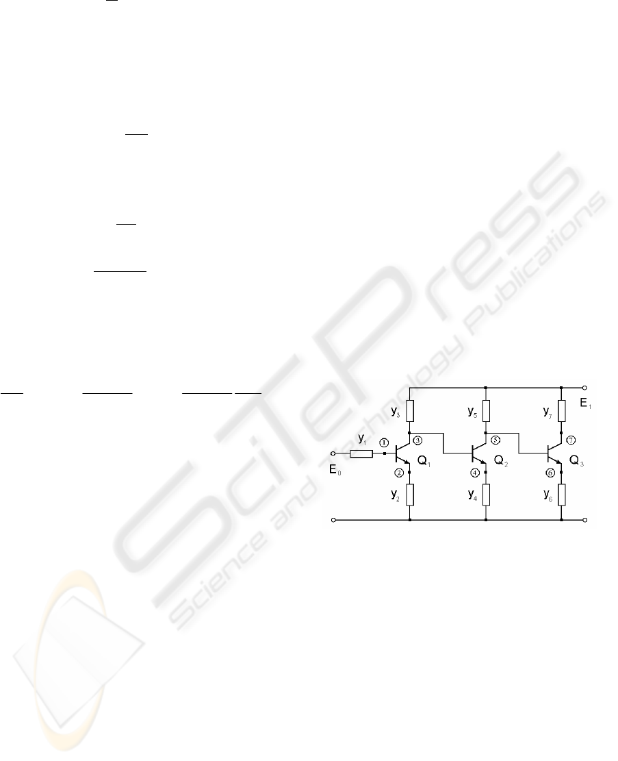
Numerical results for the transistor amplifier that is
shown in Fig. 1 are discussed below.
Figure 1: Circuit topology for three-cell transistor
amplifier.
The Ebers-Moll static model of the transistor has
been used. The analyzed circuit has seven
admittance as independent variables
7654321
,,,,,, yyyyyyy , (K=7) and seven nodal
voltages as dependent variables
7654321
,,,,,, VVVVVVV
,
(M=7).
The results of the analysis of the traditional
design strategy and some other strategies that have
the computer time less than the traditional strategy
are given in Table 1. The first line corresponds to the
TDS. The last line corresponds to the MTDS. Other
nes are the intermediate strategies. The optimal
strategies from this table (number 18 and 25 for two
optimization procedures respectively) are not
optimal in general and the data for the time-optimal
GENERAL FORMULATION OF SYSTEM DESIGN PROCESS - Design Process Formulation as a Controllable Dynamic
System
345

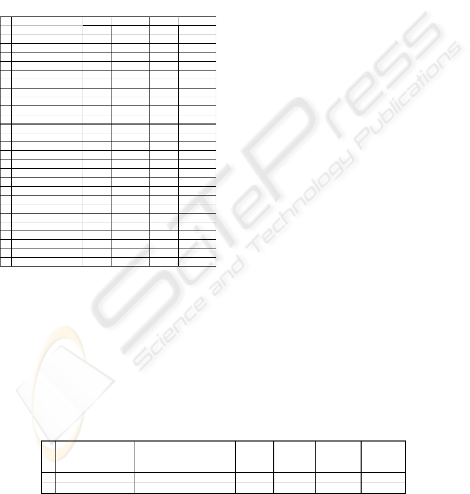
strategies are given in Table 2 by means of the
control vector variation.
The time gain of the optimal design strategy with
respect to the traditional strategy is equal to 285 for
the gradient method and 200 for the DFP method.
These data show good perspectives for proposed
approach. However the potential time gain is
realized only in case when we found the algorithm
for the optimal control vector construction.
Table 1: Data of some strategies.
5 CONCLUSIONS
The traditional approach for the analogue circuit
design is not time-optimal. The problem of the time-
optimum design algorithm can be solved adequately
on the basis of the control theory application. The
construction of the time-optimal design algorithm is
formulated as the problem of a functional
minimization of the control theory. This approach
can reduce considerably the total computer time for
the system design. Analysis of the different
electronic systems gives the possibility to conclude
that the potential computer time gain of the time-
optimal strategy increases when the size and
complexity of the system increase. The proposed
approach gives the possibility to find the time-
optimal algorithm as a solution of the typical
problem of the optimal control theory. The optimal
structure of the control vector can be finding by the
approximate methods of control theory.
ACKNOWLEDGEMENTS
This work was supported by the Mexican National
Council of Science and Technology – CONACYT,
under project SEP-2004-C01-46510.
REFERENCES
Osterby, O., Zlatev, Z., 1983. Direct Methods for Sparse
Matrices, Springer-Verlag, N.Y.
George, A., 1984. On Block Elimination for Sparse Linear
Systems, SIAM J. Numer. Anal. vol. 11, no.3, pp. 585-
603.
Wu, F.F., 1976. Solution of Large-Scale Networks by
Tearing”, IEEE Trans. Circuits Syst., vol. CAS-23, no.
12, pp. 706-713.
Sangiovanni-Vincentelli, A., Chen, L.K., Chua, L.O.,
1977. An Efficient Cluster Algorithm for Tearing
Large-Scale Networks, IEEE Trans. Circuits Syst.,
vol. CAS-24, no. 12, pp. 709-717.
Kashirsky, I.S., Trokhimenko, Y.K., 1979. The
Generalized Optimization of Electronic Circuits,
Tekhnika, Kiev.
Rizzoli, V., Costanzo, A., Cecchetti, C., 1990. Numerical
Optimization of Broadband Nonlinear Microwave
Circuits, IEEE MTT-S Int. Symp., vol. 1, pp. 335-338.
Ochotta, E.S., Rutenbar, R.A., Carley, L.R., 1996.
Synthesis of High-Performance Analog Circuits in
ASTRX/OBLX, IEEE Trans. on CAD, vol.15, no. 3,
pp. 273-294.
Zemliak, A., 2005. Generalization of Analog System
Design Methodology, In Proc. 5th WSEAS Int. Conf.
on Instrumentation, Measurement, Control, Circuits
and Syst., Cancun, Mexico, pp.114.119.
Table 2: Data of the optimal design strategies.
N Control functions Gradient method DFP method
vector Iterations Total design Iterations Total design
U (u1,u2,u3,u4,u5,u6,u7) number time (sec) number time (sec)
1 ( 0 0 0 0 0 0 0 ) 6379 321.09 854 64.47
2 ( 0 0 1 0 1 0 1 ) 922 54.53 764 52.29
3 ( 0 0 1 0 1 1 0 ) 1667 80.71 650 46.13
4 ( 0 0 1 0 1 1 1 ) 767 35.35 426 22.68
5 ( 0 0 1 1 1 0 0 ) 3024 159.67 940 52.71
6 ( 0 0 1 1 1 0 1 ) 823 37.73 177 7.71
7 ( 0 0 1 1 1 1 0 ) 3068 86.87 450 14.56
8 ( 0 0 1 1 1 1 1 ) 553 15.75 170 6.93
9 ( 0 1 1 0 1 0 1 ) 465 10.01 101 2.66
10 ( 0 1 1 0 1 1 0 ) 1157 31.92 111 3.85
11 ( 0 1 1 0 1 1 1 ) 501 8.82 124 2.66
12 ( 0 1 1 1 1 0 0 ) 2643 72.66 314 9.24
13 ( 0 1 1 1 1 0 1 ) 507 9.24 170 4.62
14 ( 0 1 1 1 1 1 0 ) 3070 67.27 423 12.25
15 ( 1 0 1 0 1 0 1 ) 1345 28.07 397 16.94
16 ( 1 0 1 0 1 1 1 ) 615 10.01 191 4.62
17 ( 1 0 1 1 1 0 1 ) 699 10.71 197 4.97
18 ( 1 0 1 1 1 1 1 ) 366 4.97 103 1.96
19 ( 1 1 1 0 1 0 1 ) 789 10.43 201 4.97
20 ( 1 1 1 0 1 1 0 ) 3893 61.53 1158 18.06
21 ( 1 1 1 0 1 1 1 ) 749 7.71 148 2.11
22 ( 1 1 1 1 1 0 0 ) 4325 90.72 945 19.18
23 ( 1 1 1 1 1 0 1 ) 796 8.47 133 2.31
24 ( 1 1 1 1 1 1 0 ) 2149 29.26 1104 13.44
25 ( 1 1 1 1 1 1 1 ) 2031 5.67 180 0.77
N Method Optimal control Iterations Switching Total Computer
functions vector number points design time gain
U (u1,u2,u3,u4,u5,u6,u7) time (sec)
1 Gradient method (1111111); (1111101) 363 350 1.127 285
2 DFP method (1111111); (1110111) 69 66 0.322 200
ICINCO 2007 - International Conference on Informatics in Control, Automation and Robotics
346