
TRAJECTORY PLANNING USING OSCILLATORY CHIRP
FUNCTIONS APPLIED TO BIPEDAL LOCOMOTION
Fernando Juan Berenguer Císcar
Escuela Superior Politécnica, Universidad Europea de Madrid,C/ Tajo s/n, Villaviciosa de Odón, Spain
Félix Monasterio-Huelin Maciá
E.T.S.I. de Telecomunicación,Universidad Politécnica de Madrid, C/ Ciudad Universitaria s/n, Madrid, Spain
Keywords: Trajectory planning, bipedal walking robot, chirp functions.
Abstract: This work presents a method for planning sinusoidal traj
ectories for an actuated joint, so that the oscillation
frequency follows linear profiles, like trapezoidal ones, defined by the user or by a high level planner. The
planning method adds a cubic polynomial function for the last segment of the trajectory in order to reach a
desired final position of the joint. We apply this planning method to an underactuated bipedal mechanism
which gait is generated by the oscillatory movement of its tail. Using linear frequency profiles allow us to
modify the speed of the mechanism and to study the efficiency of the system at different speed values.
1 INTRODUCTION
Trapezoidal and linear velocity profiles are widely
used in trajectory planning for mobile robots and
robot manipulators. The necessary procedure for
defining this kind of trajectories can be found in
many robotic textbooks (Spong, 1989, Sciavicco,
1996, Craig, 2006). In other robotic areas, as in the
case of walking machines and nonholonomic
locomotion systems, the robot joints execute
oscillatory motions, and some planning methods are
based on using sinusoidal trajectories with constant
frequencies (Morimoto, 2006, Sfakiotakis, 2006,
Murray, 1993). In (Berenguer, 2006) we presented
an underactuated bipedal mechanism that is able to
walk using only one actuator that moves a tail
following a sinusoidal trajectory. The displacement
velocity of these systems depends on the oscillation
frequencies together with other parameters. The
planning method presented here provides continuous
sinusoidal joint trajectories that follow desired
piecewise-linear frequency profiles and generate
smooth variation of the systems speed.
On the other hand, swept sinusoids (chirps) are
usu
ally used for identifying and modelling actuators
and mechanisms (McClung, 2004, Leavitt, 2006). In
this work, we estimate the optimal stride frequency
of a biped by means of analyzing the step length at
different frequencies, during the execution of a
trajectory generated by the proposed planning
method.
This paper is organized as follows. Next section
p
resents an initial example problem and shows
perhaps a common beginner’s mistake in the way of
solving this problem. The correct problem’s solution
is also provided in this section. Section III sets out
the planning problem in a general form and presents
the proposed solution method. Section IV shows the
application of this method to a bipedal model and
how we can use the results for analyzing the
efficiency of the model at different speeds. Finally,
section V presents conclusions and future work.
2 AN INITIAL EXAMPLE
Suppose we want to generate a sinusoidal trajectory
with unit amplitude for a robot joint. The joint is
initially at its central position (0rad) with zero
velocity, and will start to oscillate with an increasing
frequency. The joint must reach a frequency of
πrad/s at instant t=10s and keep this value during 20
seconds. Finally, the joint must reduce its frequency
to zero and achieve the central position again at
70
Juan Berenguer Císcar F. and Monasterio-Huelin Maciá F. (2007).
TRAJECTORY PLANNING USING OSCILLATORY CHIRP FUNCTIONS APPLIED TO BIPEDAL LOCOMOTION.
In Proceedings of the Fourth Inter national Conference on Informatics in Control, Automation and Robotics, pages 70-75
DOI: 10.5220/0001643600700075
Copyright
c
SciTePress
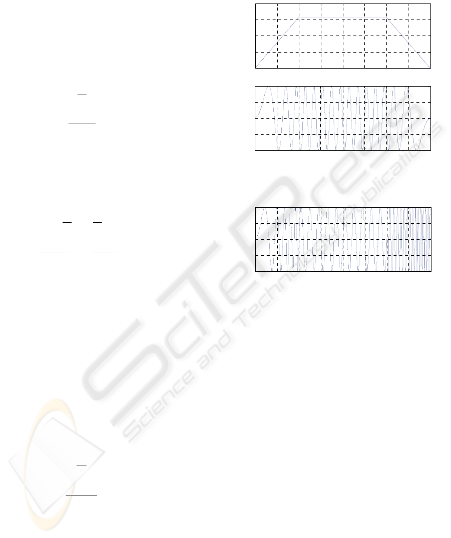
instant t=40s. Figure 1 shows this trapezoidal
frequency profile and a continuous joint trajectory
q(t) that follows it and finishes at zero position.
As a first solution to this problem, a beginner
might propose the expression in (1) for the joint
trajectory q(t). This is a sine function and we can
check that the function ω(t) follows the trapezoidal
profile.
⎪
⎪
⎩
⎪
⎪
⎨
⎧
≤<
−
π
<≤π
<≤π
=ω
ω=
40t30
10
)t40(
30t10
10t0
10
t
)t(
where)t)t(sin()t(q
(1)
Figure 2 shows this function (1) and of course
this is not the correct solution. We can see the reason
for this result by analyzing the time derivative
given by (2).
)t(q
⎪
⎪
⎩
⎪
⎪
⎨
⎧
≤≤
−
π
−
π
<≤ππ
<≤ππ
=
40t30)t
10
)t40(
cos(
10
)t240(
30t10)tcos(
10t0)
10
t
cos(
10
t
2
)t(q
2
(2)
First, at instant t=10s, the left value of is
twice as much as the right value, and we can see this
effect in the slope change of q(t) in figure 2. We find
a similar result at time t=30s, where there is a
discontinuity in from π to -2π. It is also
unexpected that increases during the last
trajectory segment and at t=40s, when ω(t)=0rad/s
and we expected zero velocity, its value is -4π rad/s.
)t(q
)t(q
)t(q
The right solution for this example problem is
(3), where θ(t) is the phase of the sinusoidal
function, and its time derivative also follows
the trapezoidal profile in figure 1.
)t(θ
⎪
⎪
⎩
⎪
⎪
⎨
⎧
≤≤
−
π
<≤π+π
<≤π
=θ
θ=
40t30
20
)t40(
30t10t
10t0
20
t
)t(
where))t(sin()t(q
2
2
(3)
Using (3) the final value of q(t) is the desired
zero value. In a general problem, a desired final
value of q(t) can’t be reached if we use only linear
functions in the profile and impose time instants and
frequency values. We will see that we need another
degree of freedom using, for example, a last
quadratic function in the profile, to obtain a desired
final value for the sinusoidal trajectory.
0 5 10 15 20 25 30 35 40
0
1
2
3
4
Time (s)
Radian frequency (rad/s)
0 5 10 15 20 25 30 35 40
-1
-0.5
0
0.5
1
Time (s)
Joint position (rad)
(a)
(b)
Figure 1: (a) Desired trapezoidal frequency profile and (b)
desired trajectory for an actuated robot joint.
0 5 10 15 20 25 30 35 40
-1
-0.5
0
0.5
1
Time (s)
Joint position (rad)
Figure 2: Graphical representation of function (1).
2.1 Basic Definitions
Given a sinusoidal function (sine or cosine) like (4),
the argument θ(t) is the instantaneous phase and its
time derivative is the instantaneous radian
frequency. When θ(t) varies linearly with time, its
time derivative is constant and its value is the radian
frequency, as in the time interval [10s, 30s] in (3).
(
)
)t(sinA)t(f
θ
=
(4)
When the phase is quadratic, as in the first and
last intervals in (3), the instantaneous radian
frequency varies linearly between two values and
f(t) is called a chirp function. So, the profile in
figure 1 shows the instantaneous radian frequency of
a sinusoidal function and represents the
concatenation of chirp functions. We will consider
here constant frequency sinusoids as a subset of
chirp functions, with the same initial and final
frequencies.
TRAJECTORY PLANNING USING OSCILLATORY CHIRP FUNCTIONS APPLIED TO BIPEDAL LOCOMOTION
71

3 INTERPOLATION OF CHIRP
FUNCTIONS
We now present a method for planning trajectories
without discontinuities in the joint position and
velocity by means of the concatenation of chirp
functions. First we obtain the solution without a
desired final position, and in section 3.1 we add this
constraint to the problem and solve it using a final
cubic phase function.
Problem statement: Given a set of N+1 time
instants t
i
(for i=1 to N+1), and a set of N+1 desired
radian frequencies ω
i
at each instant t
i
, find a set of
N chirp functions f
i
(t) so that their concatenation
represents a continuous trajectory with amplitude A,
initial value q(t
1
)=q
1
, and which instantaneous
frequency interpolates the frequencies ω
i
.
To solve this problem, we will use the function
family given by (5).
()
⎪
⎩
⎪
⎨
⎧
≤
<≤+−+−
<
=θ
θ=
+
+
tt0
tttc)tt(b)tt(a
tt0
)t(
where)t(sinA)t(f
1i
1iiiii
2
ii
i
i
ii
(5)
The problem centres on finding the coefficients
of the phases θ
i
(t), and it is basically the same
problem of interpolating trajectories with linear
velocity profiles.
The set of conditions that allow us to solve this
problem is:
ii1ii1i1ii
iiii
ii1iii
1111
b)tt(a2)t(
b)t(
c)t()t(
c)A/qarcsin()t(
+−=ω=θ
=ω=θ
=θ=θ
==θ
+++
−
(6)
From these expressions, the values of a
i
and b
i
are directly calculated, and the c
i
coefficients, that
represent the initial phase in each profile’s segment,
must be calculated iteratively:
1i1ii1i
2
1ii1ii
11
ii
i1i
i1i
i
c)tt(b)tt(ac
)A/)t(qarcsin(c
b
)tt(2
a
−−−−−
+
+
+−+−=
=
ω=
−
ω−ω
=
(7)
The main problem of this solution is that we can
not establish a desired final value of the joint
position.
3.1 Concatenation of Chirp Functions
with a Final Cubic Phase
Usually, a planned trajectory finishes with zero
velocity, and in these cases it is interesting also to
reach a desired joint position q
N
. This condition adds
a new constraint for selecting the last trajectory
function f
N
(t) and therefore the phase θ
N
(t) needs
another degree of freedom, that is, we need to use a
cubic function instead of a quadratic one:
(
)
⎪
⎩
⎪
⎨
⎧
≤
<≤+−+−+−
<
=
=θ
θ
=
+
+
tt0
tttn)tt(m)tt(l)tt(k
tt0
)t(
where)t(sinA)t(f
1N
1NNN
2
N
3
N
N
N
NN
(8)
The set of conditions that θ
N
(t) must satisfy is:
(
)
1N1NN
NNN
N1NNN
1NNN
)t(
)t(
)t()t(
)t(sinAq
++
−
+
ω=θ
ω=θ
θ=θ
θ=
(9)
The first of these conditions has many solutions,
so we will find the solution corresponding to an
almost linear profile, that is, the final phase value
will be the nearest to the final value that we will
obtain from (7) for i=N. To obtain the coefficients k,
l, m and n, we use the next procedure:
1-. First, we calculate the final phase in the quadratic
case using the coefficients a
N
, b
N
and c
N
obtained
from (7), and also the integer number of revolutions
around the unit circle:
NN1NN
2
N1NNquad
c)tt(b)tt(a +−+−=θ
++
(10)
(
)
π
θ
=
2/floorr
quad
(11)
2-. Next, we select an angle α
∈
[0, 2π), in the same
side of the unit circle as θ
quad
, that satisfies the first
condition in (9).
⎩
⎨
⎧
≥θ
<θ−π
=α
0)cos()A/qarcsin(
0)cos()A/qarcsin(
quadN
quadN
(12)
If α<0, we will add 2π (α=α+2π).
3-. The desired phase at t
N+1
is then given by (13).
ICINCO 2007 - International Conference on Informatics in Control, Automation and Robotics
72
π+α
=
θ=θ
++
r2)t(
1N1NN
(13)
4-. Finally, we calculate the coefficients by means of
(14). These expressions are obtained from (13) and
the last three conditions in (9).
3
N1N
N1N1NNN1N1N
2
N1N
N1N1NNN1N1N
N
N1N
)tt(
)tt)(())t((2
k
)tt(
)tt)(2())t((3
l
m
)t(n
−
−ω+ω+θ−θ−
=
−
−ω+ω−θ−θ
=
ω=
θ=
+
++−+
+
++−+
−
(14)
4 APPLICATION TO AN
UNDERACTUATED BIPEDAL
MECHANISM
We now present experimental results from
simulations where we apply this trajectory planning
method to a bipedal walking model. This model is
described in more detail in (Berenguer, 2007), and
we now include a brief description.
4.1 Bipedal Model and Gait
Descriptions
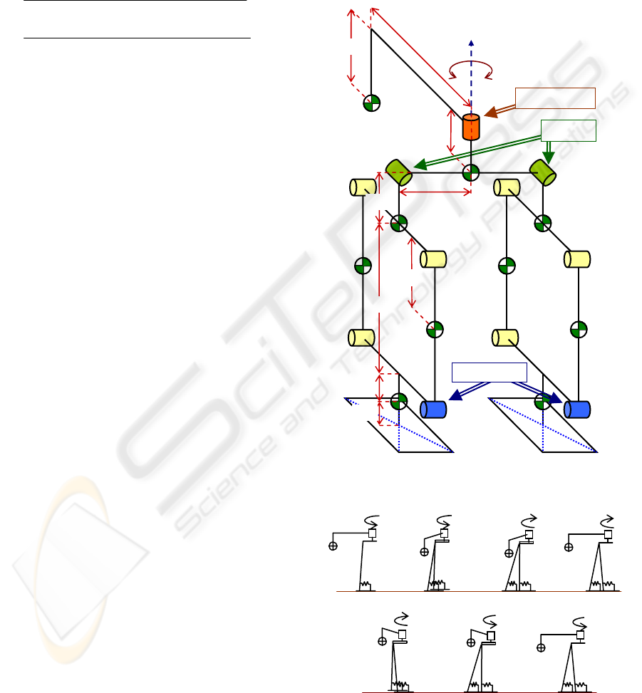
The walking model, shown in figure 3, consists of a
light body, a tail connected to it and two legs. Each
leg is formed by a parallel link mechanism and a flat
rectangular foot. The tail, with an almost horizontal
displacement, works as a counterbalance and
controls the movement of the biped.
The joint connecting the tail to the body is
actuated by an electric motor and it is the only
actuated degree of freedom. Connecting the body to
each leg are the top joints. Their rotation axis is
normal to the frontal plane, so they allow the
mechanism to raise a foot while both feet remain
parallel to the ground. These top joints are passive
joints with negligible friction. Finally, each parallel
link mechanism has four joints, and we consider that
in one of these joints (the ankle joint) there is a
spring with friction. Due to the characteristics of the
parallel link mechanism, these four joints represent
only one passive degree of freedom for each leg of
the mechanism. In summary, the model has eleven
joints, four passive degrees of freedom and one
actuated degree of freedom.
We now describe how the mechanism can walk
when the tail moves side to side in an oscillating
way. We start by supposing that the biped is at an
equilibrium position with the tail in its central
position (Fig.4.a). Both ankle springs hold the
weight of the mechanism and it stays almost vertical.
When the tail moves to a lateral position of the
mechanism, its mass acts as a counterbalance and
produces the rise of one of the feet (Fig.4.b). Then
only one spring holds the body, so the stance leg
falls forward and the swing leg moves forward as a
pendulum until the foot contacts the ground (fig.4.c).
Figure 3: Model of the biped mechanism.
Figure 4: Phases during a stride.
(a)
(b)
(c)
(d)
(e)
(f) (g)
Top joints
q(t)
Actuated joint
Ankle joints
150mm
35mm
20mm
50mm
200mm
400mm
5mm
5mm
30mm
700gr
50gr
50gr
200gr
200gr
200gr
TRAJECTORY PLANNING USING OSCILLATORY CHIRP FUNCTIONS APPLIED TO BIPEDAL LOCOMOTION
73

During the new double support phase, the tail
moves to the other side and the ankle springs move
the body backwards (fig.4.d). When the tail reaches
the other side, the second foot rises and a new step is
generated (fig.4.e). In this single support phase, the
spring of the foot that is in the ground produces
enough torque to take the body forward again. This
second step finishes with a new contact of the swing
leg with the ground (fig.4.f).
Figure 4.g represents the last instant of this initial
stride, and the starting point of a new one or the final
configuration of a completed trajectory. We can see
that if the tail stops, the system will stay in a steady
configuration with no energy cost.
4.2 Example of Trajectory Generation
We want to design a trajectory that allows us to
evaluate and analyze the biped behaviour at three
different oscillation frequencies. The frequency
profile must achieve these frequencies in a linear
way, and keep them during some periods, so we can
suppose a quasi-periodic gait at the end of each
constant frequency segment. The desired oscillation
amplitude is 1.5 rad and the radian frequencies and
time instants are:
[]
{
}
[]
{
3002001601409070200st
05.15.1115.05.00s/rad
i
i
=
=ω
}
(15)
Using (7) we obtain q(t) with a linear profile shown
in figure 5.
()
180)200t(5.1)200t(0075.0)t(
120)160t(5.1)t(
95)140t()140t(0125.0)t(
45)90t()t(
30)70t(5.0)70t(0125.0)t(
5)20t(5.0)t(
t0125.0)t(
tttat)t()t(
)t(sin5.1)t(q
2
7
6
2
5
4
2
3
2
2
1
1iii
+−+−−=θ
+−=θ
+−+−=θ
+−=θ
+−+−=θ
+−=θ
=θ
<≤θ=θ
θ=
+
(16)
As we can see in figure 6, this solution provides
the final joint position q(300)= -0.76rad. If the
desired final tail position is q=0rad, it will be
necessary to apply the procedure in section 3.1. The
solution in this case is the same as in (16) but with
the last phase θ
7
(t) given by:
180)200t(5.1)200t(10659.7
)200t(10062.1)t(
23
36
7
+−+−×+
+−×=θ
−
−
(17)
Figure 5 shows the frequency profiles of both
solutions. We can see a most linear segment in the
last time interval for the second solution which
practically overlaps the first solution’s profile.
Figure 6 shows both trajectories nearly overlapping
during the last time interval, with the same number
of oscillations but different final value.
0 50 100 150 200 250 300
0
0.5
1
1.5
Time (s)
Figure 5: Instantaneous frequency profiles.
Figure 6: Trajectory of the tail joint.
4.3 Evaluation of the Mechanism
Behaviour
The bipedal mechanism walks with a forward speed
which is proportional to the stride length and
frequency. The stride frequency is the same as the
tail oscillation frequency and the stride length
depends on the tail frequency and also on other
parameters of the model. If we fix the values of
these other parameters, the speed and energy
consumption of the mechanism will depend in a non
linear way on the stride frequency. Using linear
frequency profiles we can analyze this dependency
and estimate a near optimal joint frequency for an
established set of model parameters.
Figure 7 shows the distance covered by the biped
and the mechanical energy required by the tail joint
during the execution of the last trajectory defined in
section 4.2. The relative small amplitude oscillations
are due to the forward and backward oscillation of
the body during walking. The mechanical energy has
been calculated by the integration of the absolute
value of the product between the angular velocity of
the joint and the required torque. We observe an
important difference in the walking speed for the
first and second oscillation frequencies, and a much
Frequency (rad/s)
0 50 100 150 200 250 300
-1.5
-1
-0.5
0
0.5
1
1.5
Time (s)
Tail joint position (rad)
ICINCO 2007 - International Conference on Informatics in Control, Automation and Robotics
74

smaller variation for the second and third ones,
while the power consumption varies significantly for
these last frequencies. So, we find a loss of
efficiency when we increment the stride frequency.
Table 1 presents numerical data considering the
last stride period just before a change in the
oscillation frequency. We suppose that the gait is
almost periodic during this last period. Figure 8
shows these values and also an estimation of the
same magnitudes at different frequencies. This
estimation is obtained from the last profile’s
segment, which covers all frequencies between 0
and 1.5rad/s, considering each half-oscillation as an
approximation of half-period of a sinusoid.
As we can see, speed goes up quickly at low
frequencies because stride length also grows. For
frequencies greater than 1.04rad/s, stride length
decreases with frequency and speed rises more
slowly. We also notice that speed and power have
similar behaviour (S-curve) before this frequency.
After that, the power slope increases whereas speed
slope decreases. We consider this 1.04rad/s
frequency as a near optimal oscillation frequency for
the actuated joint.
Table 1: Stride length, speed and mechanical power at
three different stride frequencies during a stride.
Stride
frequency
(rad/s)
Stride
period
(s)
Stride
length
(m)
Speed
(m/s)
x10
-3
Power
(W)
x10
-3
0.5 12.57 0.0807 6.422 1.386
1.0 6.283 0.1992 31.704 10.707
1.5 4.188 0.1767 42.184 18.694
Figure 7: Crossed distance and mechanical energy during
the trajectory execution.
0.5 1 1.5
0.05
0.1
0.15
0.2
0.25
Frequency (rad/s)
Stride length (m)
0.5 1 1.5
0
10
20
30
40
50
Frequency (rad/s)
Speed (mm/s)
0.5 1 1.5
0
5
10
15
20
Frequency (rad/s)
Mechanical Power (mW)
Figure 8: Stride length, mechanism speed and required
mechanical power at different joint frequencies.
5 CONCLUSIONS
In this work we propose a method for planning
oscillatory trajectories based on the concatenation of
chirp functions. By means of adding a final cubic
function, the joint can also reach a desired final
position following a nearly linear frequency profile.
Our aim is to apply this method to a bipedal robot
that walks moving a tail in an oscillatory way.
This planning method allows us to study the gait
efficiency at different stride frequencies during the
design and adjusting phase. On the other hand, the
implementation of this planner will allow a real
prototype to select the forward speed as a function of
the obstacles density, ground inclination or for
optimization requirements.
REFERENCES
Spong, M. W., Vidyasagar, M., 1989, Robot Dynamics
and Control, John Wiley & Sons.
Sciavicco, L., Siciliano, B., 1996. Modeling and Control
of Robot Manipulators, The McGraw-Hill Comp., 1
st
edition.
Craig, J. J., 2006. Introduction to robotics, Prentice Hall,
3
th
edition.
Morimoto, J., Gen Endo, Jun Nakanishi, Hyon, S., Cheng,
G., Bentivegna, D., Atkeson, C.G., 2006, “Modulation
of simple sinusoidal patterns by a coupled oscillator
model for biped walking”, in Proc. 2006 IEEE
International Conference on Robotics and
Automation, USA, pp.1579-1584.
Sfakiotakis, M., Tsakiris, D. P., Vlaikidis, A., 2006,
“Biomimetic Centering for Undulatory Robots”, in
Proc. of the 1st IEEE Int. Conference on Biomedical
Robotics and Biomechatronics, pp.744- 749.
0 50 100 150 200 250 300
0
1
2
3
4
5
6
7
Time (s)
Crossed distance (m)
0 50 100 150 200 250 300
0
0.5
1
1.5
2
2.5
3
3.5
Time (s)
Mechanical energy (J)
Crossed distance
Mechanical energy
Murray, R. M., Sastry, S., 1993, “Nonholonomic motion
planning: Steering using sinusoids”, IEEE Trans. on
Automatic Control, 38(5), pp.700-716.
McClung, A. J., Cham, J. G., Cutkosky, M. R., 2004,
“Rapid Maneuvering of a Biologically Inspired
Hexapedal Robot” in ASME IMECE Symp. on Adv. in
Robot Dynamics and Control, USA.
Leavitt, J., Sideris, A., Bobrow, J. E., 2006, “High
bandwidth tilt measurement using low-cost sensors”,
IEEE/ASME Trans. on Mechatronics, 11(3), pp.320-
327.
Berenguer, F. J., Monasterio-Huelin, F., 2006, “Easy
design and construction of a biped walking mechanism
with low power consumption”, in Proc. of
CLAWAR’06, the 9th Int. Conference on Climbing and
Walking Robots, Belgium, pp. 96-103.
Berenguer, F. J., Monasterio-Huelin, F., 2007, “Stability
and Smoothness Improvements for an Underactuated
Biped with a Tail”, in Proc. of the 2007 IEEE Int.
Symposium on Industrial Electronics, Vigo, Accepted.
TRAJECTORY PLANNING USING OSCILLATORY CHIRP FUNCTIONS APPLIED TO BIPEDAL LOCOMOTION
75
