
APPLICATIONS OF A MODEL BASED PREDICTIVE CONTROL
TO HEAT-EXCHANGERS
Radu Bălan, Vistrian Mătieş, Victor Hodor
Dept.of Mechatronics, Technical University of Cluj-Napoca, C. Daicoviciu no. 15, Cluj-Napoca, Romania
Sergiu Stan, Ciprian Lăpuşan, Horia Bălan
Dept. of Mechanics and Programming, Dept.of Mechatronics, Dept. of Energetics, Technical University of Cluj-Napoca
Keywords: Heat-exchanger, nonlinear control, on-line simulation, rule-based control.
Abstract: Model based predictive control (MBPC) is an optimization-based approach that has been successfully
applied to a wide variety of control problems. When MBPC is employed on nonlinear processes, the
application of this typical linear controller is limited to relatively small operating regions. The accuracy of
the model has significant effect on the performance of the closed loop system. Hence, the capabilities of
MBPC will degrade as the operating level moves away from its original design level of operation. This
paper presents an MBPC algorithm which uses on-line simulation and rule-based control. The basic idea is
the on-line simulation of the future behaviour of control system, by using a few control sequences and based
on nonlinear analytical model equations. Finally, the simulations are used to obtain the ‘optimal’ control
signal. These issues will be discussed and nonlinear modelling and control of a single-pass, concentric-tube,
counter flow or parallel flow heat exchanger will be presented as an example.
1 INTRODUCTION
Model Based Predictive Control (MBPC) refers to a
class of algorithms that utilize an explicit process
model to compute the control signal by minimizing
an objective function (Comacho, 1999). The
performance objective typically penalizes predicted
future errors and manipulated variable movement
subject to various constraints. The ideas appearing in
greater or lesser degree in all the predictive control
family are basically:
-explicit use of a model to predict the process
output in the future;
-on line optimization of a cost objective function
over a future horizon;
-receding strategy, so that at each instant, the
horizon is displaced towards the future, which
involves the application of the first control signal of
the sequence calculated at each step.
Performance of MBPC could become
unacceptable due to a very inaccurate model, thus
requiring a more accurate model. This task is an
instance of closed-loop identification and adaptive
control. Here it is important to remember that the
model is only used as an instrument in creating the
best combined performance of the controller and the
actual system, so the model does not necessarily
need to be a good open-loop model of the system.
The performance measure should be able to capture
as much of the closed loop behavior as possible.
Let’s consider that it is possible to compute:
- the predictions of output over a finite horizon (N);
- the cost of an objective function,
for each possible sequence:
(
)
{
}
)(),..,1(),(. Ntututuu +
+
=
(1)
and then to choose the first element of the optimal
control sequence. For a first look, the advantages of
the proposed algorithm (Balan, 2001) include the
following:
-the minimum of objective function is global;
-it is not necessary to invert a matrix, so potential
difficulties are avoided;
-it can be applied to nonlinear processes if a
nonlinear model is available;
-the constraints (linear or nonlinear) can easily be
implemented.
The drawback of this scheme is a very long
computational time, because there are possibly a lot
of sequences. For example, if u(t) is applied to the
296
B
ˇ
alan R., M
ˇ
atie¸s V., Hodor V., Stan S., L
ˇ
apu¸san C. and B
ˇ
alan H. (2007).
APPLICATIONS OF A MODEL BASED PREDICTIVE CONTROL TO HEAT-EXCHANGERS.
In Proceedings of the Fourth International Conference on Informatics in Control, Automation and Robotics, pages 296-301
DOI: 10.5220/0001646102960301
Copyright
c
SciTePress

process using a “p” bits numerical-analog converter
(DAC), the number of sequences is 2
p
*
N
.Therefore,
the number of sequences must be reduced.
In the next sections, these issues will be
discussed and nonlinear modelling and control of a
single-pass, concentric-tube, counter flow heat
exchanger will be presented as an example.
2 THE MODEL OF THE
HEAT-EXCHANGER
Heat exchangers are devices that facilitate heat
transfer between two or more fluids at different
temperatures. Usually, MBPC uses a linear model
and an on-line least square algorithm (RLS) to
determine the parameters. Heat exchangers are
nonlinear processes. To apply the standard MBPC
algorithms it is possible to use multiple model
adaptive control approach (MMAC) which uses a
bank of models to capture the possible input-output
behavior of processes (
Dougherty, 2003). Other
solutions are based on neural networks and fuzzy
logic (Fischer, 1998), (Fink, 2001).
In this paper it is used an example from (Ozisik,
1985): a heat exchanger with hot fluid -engine oil at
80ºC, cold fluid - water at 20º C, by using a single-
pass counter flow (or parallel flow for some
experiments) concentric-tube. Other data and
notations: length (L): 60m, heat transfer coefficients
(k
1
=1000 W/(m
2
ºC), k
2
=80 W/(m
2
ºC)), the
temperature profile of fluids and wall (
),(
1
tzθ ,
),(
2
tzθ , ),( tz
w
θ ), specific heat (c
1
, c
2
, c
w
), cross-
sectional area for fluids flow and wall (S
1
, S
2
, S
w
),
density of fluids and wall (ρ
1
, ρ
2
, ρ
w
), flow speed of
fluids (v
1
, v
2
), transfer area (S) (fig. 1).
If physical properties (density, heat capacity,
heat transfer coefficients, flow speed) are assumed
constant, the heat exchanger model is described
using a shell energy balance as (Douglas, 1972):
-hot fluid:
() ()
() ()
[]
tztz
L
Sk
z
tz
Svc
t
tz
Sc
w
,,
,,
1
11
1111
1
111
θ−θ=
∂
θ∂
ρ−
∂
θ∂
ρ
(2)
-cold fluid:
()
(
)
() ()
[]
tztz
L
Sk
z
tz
Svc
t
tz
Sc
w
,,
,,
2
21
2222
2
222
θ−θ=
∂
θ∂
ρ+
∂
θ∂
ρ
(3)
-wall:
()
() ()( )()
[]
tzkktzktzk
L
S
t
tz
Sc
w
w
www
,,,
,
212211
θ+−θ+θ=
∂
θ∂
ρ
(4)
Using general notation θ
a(i,j)
with a=1 (hot fluid),
a=2 (cold fluid), a=w (wall), i, j discrete elements in
space respectively time, the discrete equations
corresponding to partial differential equations
(2),(3),(4) are:
Figure 1: Temperature distributions.
()()
() ()
ji
SLc
tSk
ji
z
t
v
SLc
tSk
z
t
vjiji
w
,,1
1,1,
111
1
11
111
1
111
θ
ρ
Δ
++θ
Δ
Δ
+
+
⎥
⎦
⎤
⎢
⎣
⎡
ρ
Δ
−
Δ
Δ
−θ=+θ
(5)
()()
() ()
ji
SLc
tSk
ji
z
t
v
SLc
tSk
z
t
vjiji
w
,,1
1,1,
222
2
22
222
2
222
θ
ρ
Δ
++θ
Δ
Δ
−
−
⎥
⎦
⎤
⎢
⎣
⎡
ρ
Δ
−
Δ
Δ
+θ=+θ
(6)
(
)
(
)
() ()( )()
[]
jikkjikjik
L
tS
jiji
w
ww
,,,
,1,
212211
θ++θ+θ
Δ
+
+θ=+θ
(7)
In a control application, these equations can not
be used directly because v
1
and v
2
are not constant in
time. Let’s consider next assumptions:
-the speed of fluids is limited:
v
1(min)
<v
1
<v
1(max)
;
v
2(min)
<v
2
<v
2(max)
;v
max
=max(v
1(max)
,v
2(max)
) (8)
- the fluids speed is only time-function:
v
1
=v
1
(t) , dv
1
/dz=0 , v
2
=v
2
(t) , dv
2
/dz=0 (9)
- the length of heat exchanger is divided in n
intervals: L=nΔz; (10)
- in an interval Δt, the fluids cover only a part of
Δz: n
v
v
max
Δt=Δz ; Δt < L /(nn
v
v
max
) (11)
- two variables Δz
1
, Δz
2
are using to totalize the
small fluid displacements:
Δz
1
(t+Δt)=Δz
1
(t)+v
1
Δt ;
Δz
2
(t+Δt)=Δz
2
(t)+v
2
Δt (12)
- in simulations, the displacements of the fluids
become effective only if Δz
1
>Δz or/and Δz
2
>Δz; in
these cases:
Δz
1
← Δz
1
-Δz or/and Δz
2
← Δz
2
-Δz (13)
In other words, in simulations, the continue moves
of fluids are replaced with small discrete
displacements. As a result, the heat exchanger model
is described by equations:
APPLICATIONS OF A MODEL BASED PREDICTIVE CONTROL TO HEAT-EXCHANGERS
297
()() ()
ji
SLc
tSk
SLc
tSk
jiji
w
,1,1,
111
1
111
1
11
θ
ρ
Δ
+
⎥
⎦
⎤
⎢
⎣
⎡
ρ
Δ
−θ=+θ
(14)
()() ()
ji
SLc
tSk
SLc
tSk
jiji
w
,1,1,
222
2
222
2
22
θ
ρ
Δ
+
⎥
⎦
⎤
⎢
⎣
⎡
ρ
Δ
−θ=+θ
(15)
()()
() ()( )()
[]
jikkjikjik
L
tS
jiji
w
ww
,,,
,1,
212211
θ++θ+θ
Δ
+
+θ=+θ
(16)
In a practical implementation, there are used
equations (12), (13), (14), (15), (16).
It is important the number and position of
temperature sensors. Here, it is considered that only
the inlet and outlet temperatures (hot fluid, cold fluid
and wall) and the flow rate of fluids are measured.
The temperatures inside heat exchanger are
estimated. The quality of heat exchange depends
especially by the heat transfer coefficients. These
parameters depend by temperatures, accumulation of
deposits of one kind or another on heat transfer
surface, shape of tube, etc. The temperature
distributions inside heat exchanger (process and
model) are presented in fig. 2 using notations θ
a
(i,j).
for process and Mθ
a
(i,j) for the model.
Figure 2: Process and model (counter flow) – diagrams.
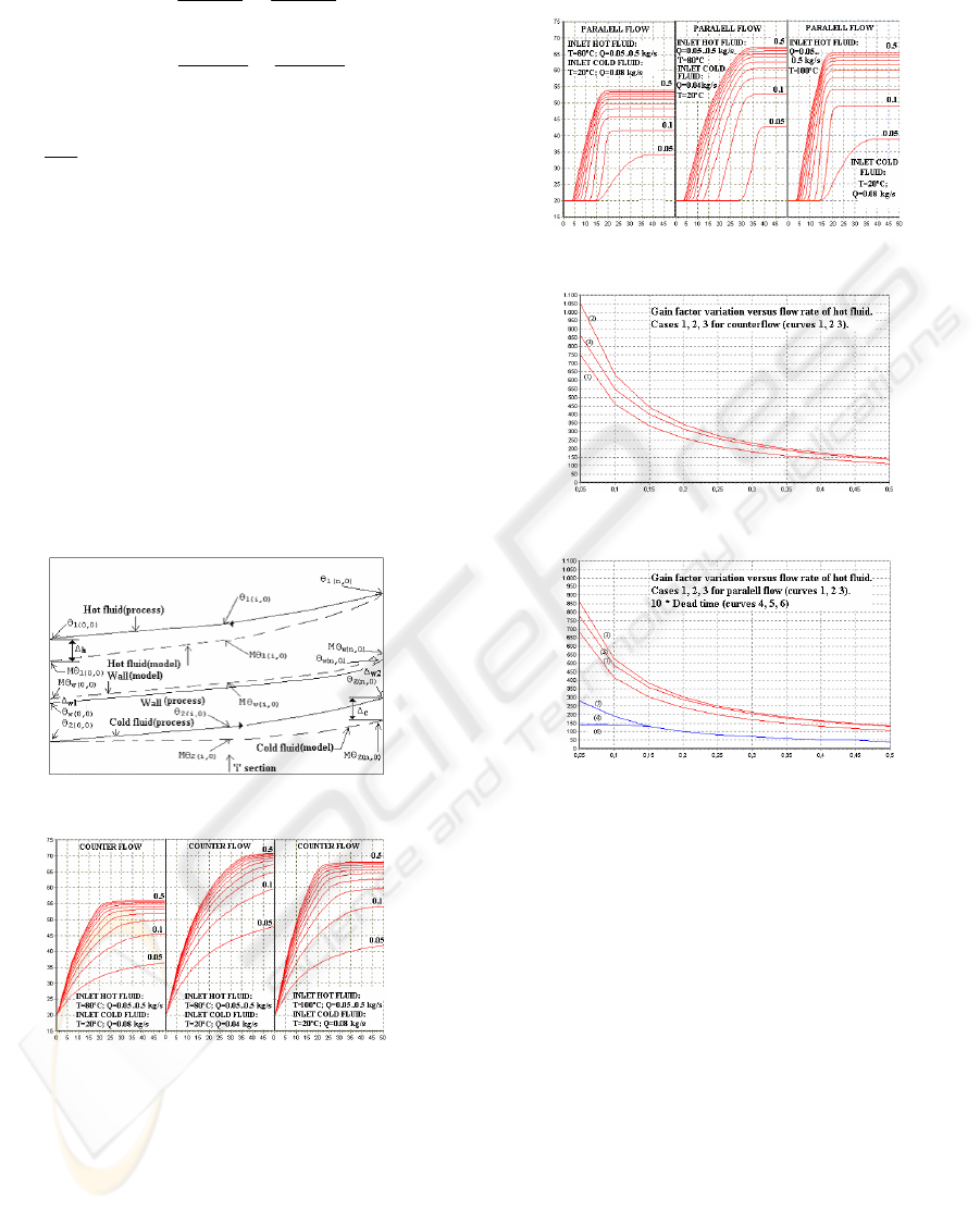
Figure 3: Step reply- counter flow.
To underline the main characteristics of the heat
exchangers that are used in simulations, there are
presented the step replies in some cases (counter
flow - fig. 3; parallel flow – fig. 4). First, the
temperatures of fluids are 20º C, than it is changed
the inlet temperature of hot fluid (input of the
process). There are different conditions for inlet
temperatures and flow rate fluids. Flow rate of hot
fluid is a parameter and permits to obtain a family of
step replies.
Figure 4: Step reply- parallel flow.
Figure 5: Counter flow- gain factor.
Figure 6: Parallel flow- gain, dead time.
Figures 5 and 6 present the dependence of gain
factor and dead time by flow rate. These simulations
underline the non-linear features of processes and,
for parallel flow, a dead time, which is dependent
especially by flow rate of hot fluid.
3 CONTROL ALGORITHM
A model based adaptive-predictive algorithm which
uses on line simulation and rule based control,
designed for linear processes, is developed in
(Balan, 2001), (Balan, 2005). This algorithm can be
applied with some modifies to nonlinear processes.
The nonlinear equations of the process can be used
directly in the control algorithm. The predictions of
system output are calculated by integrating the
nonlinear ordinary differential equations of the
model over the prediction horizon, by using a few
ICINCO 2007 - International Conference on Informatics in Control, Automation and Robotics
298
control sequences (Balan, 2005). For a first stage,
are used, the next four control sequences:
() { }
minminmin1
,..,, uuutu =
() { }
minminmax2
,..,, uuutu =
() { }
maxmaxmin3
,..,, uuutu =
() { }
maxmaxmax4
,..,, uuutu = (17)
where u
min
and u
max
are the limits of the control
signal, limits imposed by the practical constraints.
These values can depend on context and can be
functions of time. There are two pair sequences:
(u
1
(t), u
2
(t)) and (u
3
(t), u
4
(t)) which are different
through the preponderance of u
min
or u
max
in the
future control signal. The pair sequences are
different only through the first term.
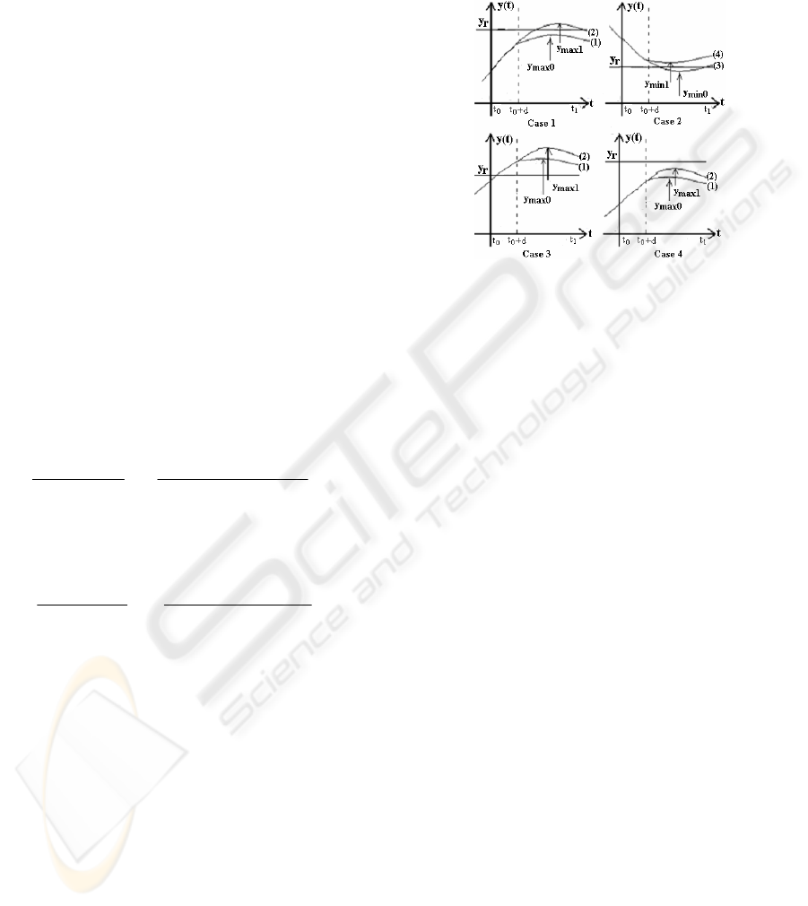
Using these sequences results four output
sequences y
1
(t), y
2
(t), y
3
(t), y
4
(t). The control signal
is computed using a set of rules based on the
extreme values y
max0
, y
max1
, y
min0
, y
min1
(fig. 7- d is
dead time, t
1
=N, y
r
is setpoint) of the output
predictions. In the followings, considering processes
with positive sign, it can be put in evidence four
usual cases:
Case 1: If y
max0
<y
r
(corresponding to u
1
(t)
sequence) and y
max1
>y
r
(corresponding to u
2
(t)
sequence) Then (using a linear interpolation):
0max1max
0maxmax1maxmin
0max1max
minmax
)(
yy
yuyu
y
yy
uu
tu
r
−
−
+
−
−
=
(18)
Case 2: If y
min0
<y
r
(corresponding to u
3
(t)
sequence) and y
min1
>y
r
(corresponding to u
4
(t)
sequence) Then (using a linear interpolation):
0min1min
0minmax1minmin
0min1min
minmax
)(
yy
yuyu
y
yy
uu
tu
r
−
−
+
−
−
=
(19)
Case 3: If: y
max0
>y
r
Then u(t
0
)=u
min
(20)
Case 4: If: y
max1
<y
r
Then u(t
0
)=u
max
(21)
In fig. 7, every output prediction curve is marked
with a number which correspond to the number of
control sequence from relations (17). Similar to case
3 and case 4, there are two similarly cases if dy/dt<0
for t<t
0
. If the algorithm uses only these 6 rules, the
variance of u(t) will be large (Balan, 2001).
So, in the second stage, depended by behaviour of
the control system, are used next methods:
-an algorithm that modifies the limits of control
signal:
u
min
≤ u
minst
(t) ≤ u(t) ≤ u
maxst
(t) ≤ u
max
Δu
min
≤ Δu≤ Δu
max
(22)
For example:
(
)
(
)()()()
(
)
tytytutuftu
r
,,1,1
maxstminst1minst
−
−
=
(23)
(
)
(
)
(
)() ()
(
)
tytytutuftu
r
,,1,1
maxstminst2maxst
−
−
=
(24)
where f
1
, f
2
are functions which decrease or increase
(depended by behavior of the control system) the
difference between u
maxst
(t) and u
minst
(t).
Figure 7: Examples of output predictions.
In relations (18)..(21), the values of u
max
, u
min
are
replaced with u
minst
(t), u
maxst
(t). In the following, if is
necessary, the next relations are used:
(
)
(
)()
(
)
11
minminstminst
−
−
+
−
=
tuuktutu
ststst
(25)
(
)
(
)()
(
)
ststst
utuktutu −−
−
−
=
11
maxmaxstmaxst
(26)
where k
st
is a weight parameter and u
st
is the
estimated value of control signal in steady state. But
in some circumstancing (perturbations, inaccurate
model) the limits of control signal must increase.
Also, it is necessary to limit the minimum value of
u
maxst
(t)-u
minst
(t)>d
ust
>0, where d
ust
is a parameter of
the control algorithm.
-using the “variable setpoint“ (Balan, 2001):
y
r1
(t)=y
r
(t)+k
ref
[y(t)-y
r
(t)] (27)
where k
ref
is a weight factor
-using a filter to compute control signal
(especially in steady state regime).
This paper will be tackled only the case when the
main aim is to control the temperature of outlet cold
fluid. To do this, it is used the flow rate of hot fluid
(controller’s output). There are possible other
objectives for example to maximize the heat transfer
between fluids. First, there was used an adaptive-
predictive algorithm based on on-line simulation and
a linear model (Balan, 2001). The parameters of
model were identified on-line using least square
algorithm. This method could be applied, with poor
results, only for counter flow heat exchanger. It is
APPLICATIONS OF A MODEL BASED PREDICTIVE CONTROL TO HEAT-EXCHANGERS
299
necessary to consider the non-linear features of heat
exchanger and to use a model of the heat exchanger
based on the finite difference method. It is supposed
that initially the heat transfer coefficients are
unknown and than they are identified on-line. In
simulations, there are used three sets of finite
difference equations: process equations, model
equations, on line simulation equations.
The behaviour of heat exchanger depends by
some types of parameters:
1. Construction parameters: length of tube,
surface of heat transfer, diameters of tubes, etc.
These parameters can be considered constants.
2. Fluids parameters: density, specific heat etc.
These parameters depend by temperature and other
conditions.
3. Parameters that determine the quality of heat
exchange, especially the heat transfer coefficients.
These parameters depend by temperatures,
accumulation of deposits of one kind or another on
heat transfer surface, shape of tube, etc.
At every sample period, it is possible to compute
Δ
h
, Δ
c
, Δ
w1
, Δ
w2
, the temperature prediction errors of
outlet hot fluid, outlet cold fluid, wall (fig. 2).
These predictions can be used to correct the
temperature distributions inside the model of heat
exchanger, using translations and rotations of
distributions. Also, prediction errors can be used to
modify the parameters of the model using an
algorithm based on rules. The control scheme is
presented in fig. 8.
Figure 8: Control scheme.
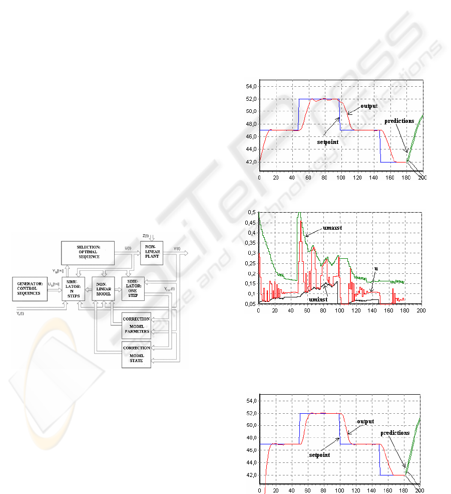
4 APPL I C ATI ONS WITH HEAT
EXCHANGERS
The next applications show the main features of the
algorithm applied to heat exchanger. The set point
has a variable shape (42°C, 47°C, 52°C, 47°C,
42°C..). The limits of u(t) (hot fluid flow rate) are:
0.05≤u(t)≤ 0.5 [kg/s]. The flow rate of cold fluid is
constant (0.08 kg/s). The temperatures of cold fluid
(
°20 ) and hot fluid ( °80 ) are constant. Some
experiments with variable flow rate or/and variable
temperature of cold fluid are presented in (Balan,
2001).
First, it is used an accurate model (Fig. 9, fig.
10). If the algorithm uses only 1..6 rules, the
variance of u(t) will be large. To reduce this
variance, a solution is to use a funnel zone for
control signal, based on inequality (22).
In steady-state regime, control signal is
computed using average of past and new values. The
algorithm do not use directly an integral component.
In figure 9, steps 50..80, the algorithm tries to reduce
the error as fast as possible. As a result, a damped
oscillation appears. To avoid this behavior, a
solution is to use a reference trajectory.
Figure 9: Setpoint, output (accurate model).
Figure 10: Controller output (accurate model).
In figure 11, 12 it is presented an adaptive case;
the heat transfer coefficients depend by temperature:
()
200/1
0
θ
+
=
kk
(28)
Figure 11: Setpoint, output (adaptive case).
ICINCO 2007 - International Conference on Informatics in Control, Automation and Robotics
300
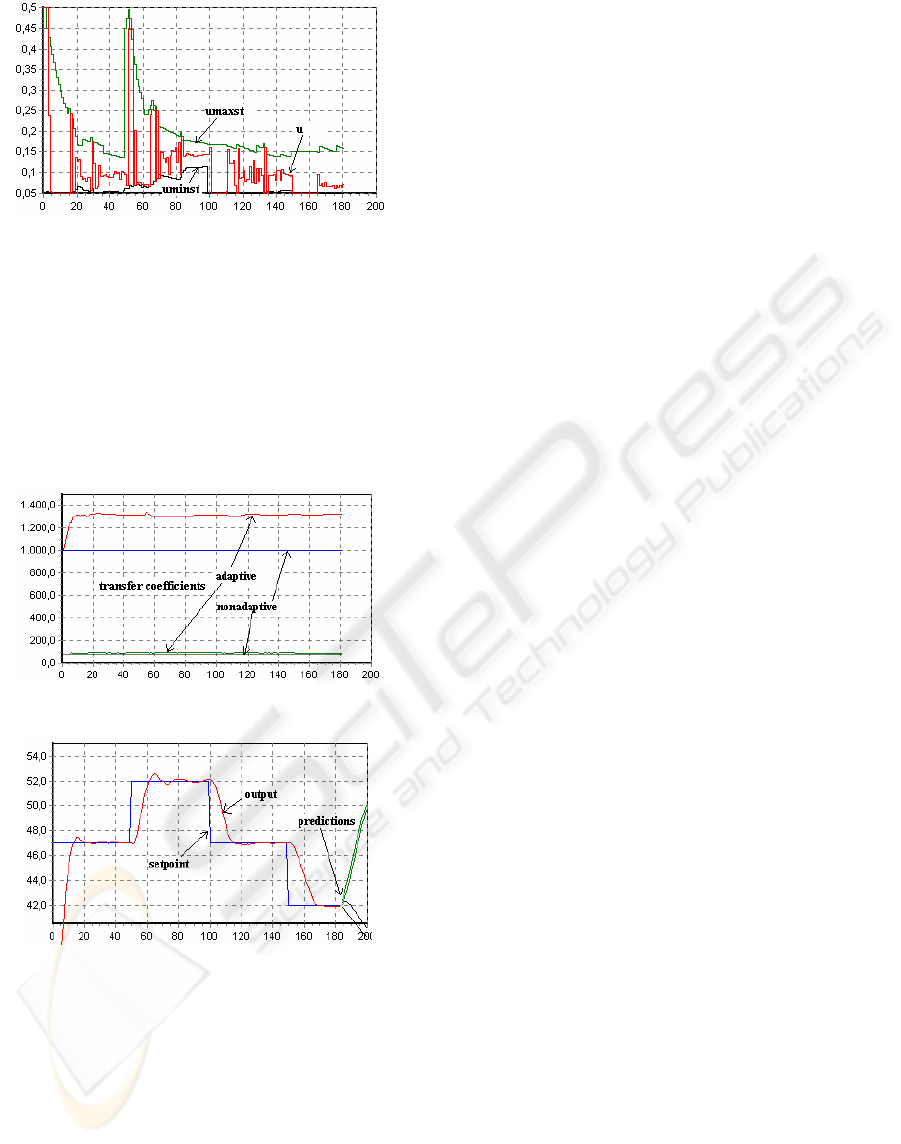
Figure 12: Controller output (adaptive case).
Initial the temperature of cold and hot fluids
is
°20 . The evolution of the estimations of heat
transfer coefficients is presented in figure 13. To
obtain these estimations, both rotations and
translations of temperature distributions and rule
based correction of heat transfer coefficients are
used. In figure 14 it is used the same conditions for
heat transfer coefficients, but it is not used this
approach.
Figure 13: Parameters identification.
Figure 14: Setpoint, output (adaptive case).
As a result, the quality of control algorithm
decreases.
5 CONCLUSION
The paper presents a simple and intuitive algorithm
applied in the case of a non linear process: heat
exchanger. A non-linear model of the process, based
on finite difference method, is used. This approach
is a numerical alternative to usual criteria equations;
offer a way to ensure the accuracy of a best-fit heat
exchanger selection, and point out that the fluids
properties must not be mathematically emphases.
Using the process model and a reduce number of the
sequences control, it is simulated the future
behaviour of the process and based on a set of rules
it is chosen the signal control considered optimum at
the actual moment. Of course there are some
difficulties such as the proof of the stability, the way
of choosing of the control sequences and the set of
rules which will lead to a better result, choosing
some parameters etc. Although, taking into account
the simplicity of this algorithm the obtained results
in the case of the presented examples by nonlinear
systems are remarkable. A demo application that
implements the proposed algorithm can be
downloaded (see web link). In the future, starting
from the proposed algorithm, the work will focus on:
the optimal chosen of the control parameters, the
study of other set of control sequences, the study of
other set of control rules, adaptive case and practical
implementation.
REFERENCES
Camacho E., Bordons C. (1999), “Model Predictive
Control” Spriger-Verlag
Radu Balan: “Adaptive control systems applied to
technological processes”, Ph.D. Thesis 2001,
Technical University of Cluj-Napoca Romania.
Dougherty, D., Cooper, D., “A practical multiple model
adaptive strategy for a single loop”, Control
Engineering Practice 11 (2003) pp. 141-159
Fischer M., Nelles O., Fink A., “Adaptive Fuzzy Model
Based Control” Journal a, 39(3), Pp22-28, 1998
Fink A., Topfer S., Isermann O., “Neuro and Neuro-Fuzzy
Identification for Model-based Control”, IFAC
Workshop on Advanced Fuzzy/Neural Control,
Valencia, Spain, Pages 111-116, 2001
Ozisik M. N., “Heat Transfer - A Basic Approach”,
McGraw-Hill Book Comp. 1985.
Douglas I.M., “Process dynamics and control”, Prentice
Hall Inc. 1972
Bălan, Radu, Vistrian Maties, Olimpiu Hancu, Sergiu
Stan, A Predictive Control Approach for the Inverse
Pendulum on a Cart Problem, IEEE-ICMA 2005 pag.
2026-2031 July 29 - August 1, 2005 Niagara Falls,
Ontario, Canada.
Available online, accessed in March, 2007:
http://zeus.east.utcluj.ro/mec/mmfm/download.htm
APPLICATIONS OF A MODEL BASED PREDICTIVE CONTROL TO HEAT-EXCHANGERS
301
