
IMAGE AND VIDEO NOISE
A Comparison of Noise in Images and Video With Regards to Detection and
Removal
Adrian J. Clark, Richard D. Green and Robert N. Grant
Dept. Computer Science, University of Canterbury, Christchurch, New Zealand
Keywords:
Image noise, motion blur, salt and pepper, video streams.
Abstract:
Despite the steady advancement of digital camera technology, noise is an ever present problem with image
processing. Low light levels, fast camera motion, and even sources of electromagnetic fields such as electric
motors can degrade image quality and increase noise levels. Many approaches to remove this noise from
images concentrate on a single image, although more data relevant to noise removal can be obtained from
video streams. This paper discusses the advantages of using multiple images over an individual image when
removing both local noise, such as salt and pepper noise, and global noise, such as motion blur.
1 INTRODUCTION
Noise is a constant frustration when dealing with
computer vision systems. While steps can be taken to
minimise noise, such as using expensive high quality
cameras and constraining operating conditions, some
noise will still be present. Low quality cameras in un-
constrained environments are more commonly being
used, and indeed are a more desirable set up for a lot
of commercial applications, and these present signifi-
cant implications for computer vision processing.
Emerging vision based technologies also bene-
fit from noise removal. Applications such as mi-
croarray imaging(Lukac et al., 2005), Medical Imag-
ing(McGee et al., 2000) and image transmission re-
quire accurate visual translations for optimal perfor-
mance. Despite previous research done in removing
noise from video streams(Kokaram, 1998) and the ad-
ditional information available in a sequence of im-
ages, the trend is still to treat noise removal on a per
image basis(Charnbolle et al., 1998).
In this paper, noise is defined to mean artefacts
within an image which are the results of inaccuracies
in capturing and converting optical information into
a digital representation. These artefacts can occur lo-
cally, such as a pixel affected by salt and pepper noise,
or globally, such as motion blur across an entire im-
age. These two types of noise can be unified as an in-
verse function of the global ambience. As the global
ambience decreases, local noise increases due to com-
pounding inaccuracies, and global noise increases due
to an increased exposure time.
2 LOCAL NOISE
We define local noise as image corruption specific to
a certain subsection of an image which is indepen-
dent of other regions of an image. This leads to a cer-
tain amount of “randomness” with the noise, such that
the noise content of a pixel cannot be accurately pre-
dicted by examining other pixels. The most common
types of local noise are Gaussian(Rank et al., 1999)
and salt-and-pepper noise(Yung et al., 1996). Salt-
and-pepper noise shows up in an image as single pix-
els with a noticeable difference in colour or intensity
from their neighbouring pixels, when in reality there
is no discernable difference between the two. Gaus-
sian noise is generally due to a low Signal to Noise
Ratio, and as the signal is lower in darker regions of
the image, noise tends to be more prevalent there.
2.1 Calibration
One major advantage of using video as opposed to a
single image for noise detection and removal is cal-
153
J. Clark A., D. Green R. and N. Grant R. (2007).
IMAGE AND VIDEO NOISE - A Comparison of Noise in Images and Video With Regards to Detection and Removal.
In Proceedings of the Second International Conference on Computer Vision Theory and Applications - IFP/IA, pages 153-156
Copyright
c
SciTePress

ibration that can be performed in additional frames.
One such approach is to use a banded light diagram,
with a gradient from dark to light. Such an artificial
diagram is computationally simple to find in a video
frame, and once found, the variance of illumination
can be determined for each light bar, using a formula
such as that shown in equation 1.
ρ = 1 −
1
N
∑
i=1
M
∑
j=1
|x
i, j
− expected|
(1)
The variance of illumination for each light level
can be used to estimate the likelihood that any given
point in future images is noise by examining the in-
tensity of it’s neighbouring pixels.
2.2 Difference of Two Images
One exploitable characteristic of gaussian noise is
that it is randomly distributed. The difference of two
consecutive frames will highlight points which have
changed between frames, including noise. Any mov-
ing objects in the scene will also show up on the im-
age, often with a far greater magnitude than noise. In
order to isolate pixels which are solely noise regions
with high difference values can be thresholded, such
that the remaining image will show many low inten-
sity pixels which are likely to be caused by noise.
2.3 Detecting Signal to Noise Ratio
Many digital web cameras have automatic white bal-
ancing and brightness controls programmed into the
firmware, which automatically adjusts the brightness,
contrast and exposure time according to light level
detected. While it is beneficial to have a consistent
brightness level, the method by which this is achieved
in the camera results in changing the Signal to Noise
Ratio. Unfortunately, many inexpensive digital cam-
eras provide no software facility for retrieving how
much light levels have been adjusted and, as shown
in Figure 1, the transition is not necessarily a smooth
gradient.
The reason for the stepping shown is unknown,
but is assumed that hysteresis is employed to pre-
vent flickering which may occur if the camera was
updating the brightness every frame. While the step-
ping does not give the exact ratio of the actual global
brightness compared to the perceived brightness, it
does provide the facility to make an assumption about
how the ratio may have changed between frames.
Figure 1: The stepping effect caused by the camera’s auto
brightness control.
2.4 Removing Local Noise
There are a range of methods available for removing
noise from an image. Typically noise is removed with
a blur or erode filter to average noisy pixels out with
neighbouring pixels. However, a global Gaussian fil-
ter can remove points which were very important for
registration or tracking, as well as reducing the inten-
sity of other significant details for computer vision,
such as edges.
A common method of avoiding this loss of de-
tail involves isolating noisy areas using a filter, and
only blurring a window around that point(Chan et al.,
2005). The approaches discussed earlier can be used
to provide points which are likely to be noisy within
images which can then be targeted by the filter.
3 BLUR
Blur is a problem encountered image processing
which can be considered in the same domain as lo-
cal noise. It is a corruption of image data which de-
grades computer vision performance. There are two
main types of blur encountered in image processing;
Static Blur which can be caused by an out of focus
camera or a damaged camera lens, and Motion Blur.
Motion blur is often present with motion under low
light levels, a problem made worse by the minimal
light capture by tiny lenses in cheaper digital cameras.
3.1 Blur Detection
A variety of algorithms have been designed to remove
motion blur, from Wiener filtering to Blind Deconvo-
lution. One common feature of all these blur removal
algorithms is that they require some sort of initial es-
timate of motion blur direction and magnitude, called
VISAPP 2007 - International Conference on Computer Vision Theory and Applications
154
a Point Spread Function (PSF), to begin the process.
While this estimate is not required to be completely
accurate, a better initial estimate will yield more ac-
curate results and a faster convergence time. Image
analysis can provide an estimate of blur characteris-
tics, but these can often be found far easier and with
higher accuracy by analysing the differences between
successive video frames using techniques such as Op-
tical Flow to estimate camera direction as shown in
figure 2.
3.2 Blur Removal
An experiment was conducted to compare deblurring
when given only a single image and when given an
image sequence. The image sequence was taken by
panning, using rotation, a typical USB web-camera,
with a resolution of 640x480 at 25 frames per second,
in an indoor laboratory environment. The camera was
rotated at approximately 150
◦
per second, providing
a 15 frame image sequence of a 90
◦
rotation.
For deblurring, the single frame method used
Blind Deconvolution algorithms while the image se-
quence used the Wiener Filter. Optical flow vectors
were extracted from the video steam and grouped ac-
cording to their direction, as shown in Figure 2. The
group with the highest count of vectors in it was cho-
sen as the most likely representative of the global di-
rection of motion. These vectors were then averaged
to create a single vector to represent direction and
magnitude of the motion.
3.3 Blur Removal Results
Due to this nature of using a real blur as opposed to a
artificially introduced one, there was no “ideal” image
for a comparison of the resulting unblurred images.
To compare the algorithms, their outputs were com-
pared visually against one another, and the motion
vectors corresponding to the cameras motion were ex-
tracted using optical flow and counted as a means of
quantitive measure. It was estimated that the Wiener
filter would produce a similar deblurring result in a
shorter amount of time than blind deconvolution, due
to the extra information available for the deblurring.
3.3.1 Image Sequence Deblurring
Deblurring the image sequence resulted in a consider-
able increase in the higher frequency components, es-
pecially in low frequency regions, such as the camels
chest. While the blurred image showed little detail
here, there is now a considerable amount of finer de-
tail, such that the fur can now be seen.
Unfortunately as a result of the deblurring, parts
of the image have begun to “ripple”, with high fre-
quency edges spreading out across the image. This is
a known effect with Wiener Filters(Jin et al., 2003),
and could be resolved by isolating the areas of de-
blurring to only lower frequency regions. The time
taken for this algorithm to run was less than ten sec-
onds, which, while not real time, could be further op-
timised. After deblurring, 233 vectors were found
over two subsequent frames which matched the an-
gle and magnitude of motion blur found in the image
sequence. The results are shown in Figure 2
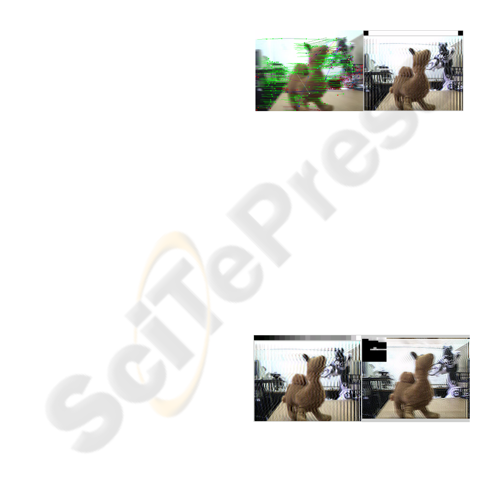
Figure 2: Left: Optical Flow vectors used to generate PSF,
Right: Image Sequence Deblurred Image.
3.3.2 Single Frame Deblurring
The blind deconvolution algorithm used was based
on the Richardson-Lucy algorithm. The accuracy of
Blind Deconvolution depends on the estimated size of
a calculated Point Spread Function. A PSF which is
too large can result in the image being deblurred too
much or even in the wrong direction, and a PSF which
is too small can result in minimal or no deblurring. To
investigate this effect the experiment was run in two
parts to examine the best case, where the estimated
size of the PSF function is exactly correct, and the
worst case where the estimated size of the PSF func-
tion is considerably incorrect. The results are shown
in Figure 3.
Figure 3: Left: Best Case Scenario and PSF above, Right:
Worst Case Scenario and PSF upper left.
IMAGE AND VIDEO NOISE - A Comparison of Noise in Images and Video With Regards to Detection and Removal
155

Table 1: Comparison of Algorithms based on Total num-
ber of points found, Percentage of found points matching
direction of motion, and time taken to perform.
Algorithm Vectors % Matching Time(s)
Wiener 491 0.47 6
Blind - Best 488 0.50 450
Blind - Worst 461 0.45 450
3.3.3 Single Frame - Best Case
For the best case scenario, the same sized PSF func-
tion that was derived from the Wiener Filter was used.
Comparing the results of the best case Blind Decon-
volution, it appears more or less on par with the re-
sults obtained from Wiener Filtering. There appears
to be a small increase in detail, but in addition, noise,
such as that appearing around the camels eye, has
been increased considerably. The time taken for the
best case scenario of Blind Deconvolution was in ex-
cess of 450 seconds, far from being realtime. The
optical flow calculation found 248 matching vectors
across two subsequent deblurred frames.
3.3.4 Single Frame - Worst Case
The experiment for Worst Case was run using the
same code as the best case, apart from the initial es-
timate of PSF size was the wrong size and shape. As
is shown in the point spread function, there appears to
be some trend in the direction of blur, but with more
noise, and thus has not deblurred correctly. The time
taken for the worst case scenario of Blind Deconvo-
lution in excess of 450 seconds. The Optical Flow al-
gorithm only found 208 matching points in the worse
case deblurring.
3.4 Blur Removal Discussion
Table 1 shows the results of the three algorithms.
Both the Wiener filter and the best case of blind de-
convolution resulted in the optical flow algorithm lo-
cating more vectors, and having similar visual clarity.
The worst case deblurring performed worse in both
the number of vectors found, and the percentage of
these which match the motion of the camera. In addi-
tion, the image appeared over-sharpened with ampli-
fied noise.
Despite the deblurring results for both video
streams and best case single images providing being
similar quality wise, the effective time taken to run the
filter for video streams was only six seconds, while
the added computation of calculating a PSF for the
single images required 450 seconds in total.
4 CONCLUSION
This paper discusses the detection and removal of
noise in video streams. Most previous research has
focused on detection and removal only in a single
frame, but in doing this useful information has been
lost about both the camera and the scene. The results
from the experiment would suggest there is validity
in processing noise based on an entire video segment,
rather than just on a frame by frame basis. In particu-
lar motion blur was looked at in detail, and an exper-
iment found that while single image deblurring can
produce results of a similar quality to that of video
the additional time required is considerable.
REFERENCES
Chan, R. H., Ho, C. H., and Nikolova, M. (2005). Salt-and-
pepper noise removal by median-type noise detectors
and detail-preserving regularization. IEEE Transac-
tions on Image Progressing, 14(10):1479–1485.
Charnbolle, A., De Vore, R., Lee, N.-Y., and Lucier, B.
(1998). Nonlinear wavelet image processing: vari-
ational problems, compression, and noise removal
through wavelet shrinkage. Image Processing, IEEE
Transactions on, 7(3):319–335.
Jin, F., Fieguth, P., Winger, L., and Jernigan, E. (2003).
Adaptive wiener filtering of noisy images and image
sequences. In Image Processing, 2003. ICIP 2003.
Proceedings. 2003 International Conference on, vol-
ume 3, pages III–349–52 vol.2.
Kokaram, A. C. (1998). Motion Picture Restoration: Dig-
ital Algorithms for Artefact Suppression in Degraded
Motion Picture Film and Video. Springer Verlag.
Lukac, R., Smolka, B., Martin, K., Plataniotis, K., and
Venetsanopoulos, A. (2005). Vector filtering for
color imaging. Signal Processing Magazine, IEEE,
22(1):74–86. TY - JOUR.
McGee, K., Manduca, A., Felmlee, J., Riederer, S., and
R.L., E. (2000). Image metric-based correction (auto-
correction) of motion effects: analysis of image met-
rics. In Journal Of Magnetic Resonance Imaging,
pages 174–181.
Rank, K., Lendl, M., and Unbehauen, R. (1999). Estimation
of image noise variance. Vision, Image and Signal
Processing, IEE Proceedings-, 146(2):80–84.
Yung, N. H. C., Lai, A. H. S., and Poon, K. M. (1996).
Modified cpi filter algorithm for removing salt-and-
pepper noise in digital images. volume 2727, pages
1439–1449. SPIE.
VISAPP 2007 - International Conference on Computer Vision Theory and Applications
156
