AN INTERPOLATION METHOD FOR THE RECONSTRUCTION
AND RECOGNITION OF FACE IMAGES
N. C. Nguyen and J. Peraire
Massachusetts Institute of Technology, 77 Massachusetts Ave, Cambridge, MA 20139, USA
Keywords:
Face reconstruction, face recognition, best points interpolation method, principal component analysis.
Abstract:
An interpolation method is presented for the reconstruction and recognition of human face images. Basic
ingredients include an optimal basis set defining a low-dimensional face space and a set of interpolation points
capturing the most relevant characteristics of known faces. The interpolation points are chosen as pixels
of the pixel grid so as to best interpolate the set of known face images. These points are then used in a
least-squares interpolation procedure to determine interpolant components of a face image very inexpensively,
thereby providing efficient reconstruction of faces. In addition, the method allows a fully automatic computer
system to be developed for the real-time recognition of faces. The advantages of this method are: (1) the
computational cost of recognizing a new face is independent of the size of the pixel grid; and (2) it allows for
the reconstruction and recognition of incomplete images.
1 INTRODUCTION
Image processing and recognition of human faces
constitutes a very active area of research. The field
has evolved rapidly and become one of the most suc-
cessful applications of image analysis and computer
vision partly because of availability of many power-
ful methods and partly because of its significant prac-
tical importance in many areas such as authenticity
in security and defense systems, banking, human–
machine interaction, image and multimedia process-
ing, psychology, and neurology. Principal component
analysis (PCA) or the Karhunen-Lo
`
eve (KL) expan-
sion is a well-established method for the representa-
tion (Sirovich and Kirby, 1987; Kirby and Sirovich,
1990; Everson and Sirovich, 1995) and recogni-
tion (Turk and Pentland, 1991) of human faces.
PCA approach (Kirby and Sirovich, 1990) for face
representation consists of computing the “eigenfaces”
of a set of known face images and approximating any
particular face by a linear combination of the leading
eigenfaces. For face recognition (Turk and Pentland,
1991), a new face is first projected onto the eigenface
space and then classified according to the distances
between its PCA coefficient vector and those repre-
senting the known faces. There are two drawbacks
with this approach. First, PCA may not handle incom-
plete data well situations in which only partial infor-
mation of an input image is available. Secondly, the
computational cost per image classification depends
on the size of the pixel grid.
This paper describes an interpolation method for
the reconstruction and recognition of face images.
The method was first introduced in (Nguyen et al.,
2006) for the approximation of parametrized fields.
The basic ingredient is a set of interpolation points
capturing the most relevant features of known face
images. The essential component is a least-squares
interpolation procedure for the very rapid computa-
tion of the interpolant coefficient vector of any given
input face. The interpolant coefficient vector is then
used to determine which face in the face set, if any,
best matches the input face. A significant advantage
of the method is that the computational cost of rec-
ognizing a new face is independent of the size of the
pixel grid, while achieving a recognition rate compa-
rable to PCA. Moreover, the method allows the recon-
struction and recognition of incomplete images.
The paper is organized as follows. In Section 2,
we present an overview of PCA. In Section 3, we ex-
91
C. Nguyen N. and Peraire J. (2007).
AN INTERPOLATION METHOD FOR THE RECONSTRUCTION AND RECOGNITION OF FACE IMAGES.
In Proceedings of the Second International Conference on Computer Vision Theory and Applications - IU/MTSV, pages 91-96
Copyright
c
 SciTePress

tend the best points interpolation method (BPIM) in-
troduced in (Nguyen et al., 2006) and apply it to de-
velop an automatic real-time face recognition system.
In section 4, we test and compare our approach with
PCA. Finally, in Section 5, we close the paper with
some concluding remarks.
2 PRINCIPAL COMPONENT
ANALYSIS
2.1 Eigenfaces
An ensemble of face images is denoted by
U
K
= {u
i
},
1 ≤ i ≤ K, where u
i
represents an i-th mean-subtracted
face and K represents the number of faces in the en-
semble. It is assumed that after proper normaliza-
tion and resizing to a fixed pixel grid Ξ of dimen-
sion N
1
by N
2
, u
i
can be considered as a vector in an
N-dimensional image space, where N = N
1
N
2
is the
number of pixels. PCA (Sirovich and Kirby, 1987;
Kirby and Sirovich, 1990) constructs an optimal rep-
resentation of the face ensemble in the sense that the
average reconstruction error
ε
∗
=
K
∑
i=1





u
i
−
k
∑
j=1
(φ
T
j
u
i
)φ
j





2
, (1)
is minimal for all k ≤ K. In the literature (Turk and
Pentland, 1991), the basis vectors φ
j
are referred as
eigenfaces and the space spanned by them is known
as the face space. The construction of the eigenfaces
is as follows.
Let U be the N × K matrix whose columns are
[u
1
,...,u
K
]. It can be shown that the φ
i
satisfy
Aφ
i
= λ
i
φ
i
, (2)
where the covariance matrix A is given by
A =
1
K
UU
T
. (3)
Here the eigenvalues are arranged such that λ
1
≥ . . . ≥
λ
K
. Since the matrix A of size N × N is large, solving
the above eigenvalue problem can be very expensive.
However, if K < N, there will be only K meaning-
ful eigenvectors and we may express φ
i
as
φ
i
=
K
∑
j=1
ϕ
ij
u
j
. (4)
Inserting (3) and (4) into (2), we immediately obtain
Gϕ
i
= λ
i
ϕ
i
, (5)
where G =
1
K
U
T
U is a symmetric positive-definite
matrix of size K by K. The eigenvalue problem (5)
Figure 1: Eigenfaces and the mean face. The mean face is
on the top left and followed by 11 top eigenfaces, in order
from left to right and top to bottom.
can be solved for ϕ
ij
,1 ≤ i, j ≤ K, from which the
eigenfaces φ
i
are obtained.
We present in Figure 1 the mean face and a few
of the top eigenfaces for a training ensemble of 400
face images extracted from the AT&T database (see
Section 4.1 for details).
2.2 Face Reconstruction
We briefly describe the reconstruction of face images
using PCA and later compare the results with those
obtained using our method. First, we project an input
face u onto the face space Φ
k
= span{φ
1
,...,φ
k
} to
obtain
u
∗
=
k
∑
i=1
a
i
φ
i
, (6)
where for i = 1,...,k,
a
i
= φ
T
i
u . (7)
We also define the associated error as
ε
∗
= ku− u
∗
k . (8)
Note that the mean face of the ensemble
U
K
should
be added to u
∗
to obtain the reconstructed image; and
that if k is set equal to K, the reconstruction is exact
for all members of the ensemble.
2.3 Face Recognition
We briefly describe the eigenface recognition proce-
dure of Turk and Pentland (Turk and Pentland, 1991).
To classify an input image, one first obtains PCA co-
efficients a
i
,1 ≤ i ≤ k, as described above. One then
computes the Euclidean distances between its PCA
coefficient vector a = [a
1
,...,a
k
]
T
and those repre-
senting each individual in the training ensemble. De-
pending on the smallest distance and the PCA recon-
struction error ε
∗
, the image is classified as belonging
to a familiar individual, as a new face, or a non-face
image. Several variants of the above procedure are
possible via the use of a different classifier such as the

nearest-neighbor classifier and a different norm such
as L
1
norm or Mahalanobis norm (Delac et al., 2005).
It is generally observed that the recognition per-
formance is improved when using a larger k. Typ-
ically, the number of eigenfaces k required for face
recognition varies from O(10) to O(10
2
) and is much
smaller than N. We note that classification of an in-
put image requires the evaluation of PCA coefficients
according to (7). The computational cost per image
classification is thus at least O(Nk). This cost de-
pends linearly on N and is quite acceptable for a small
number of input images. However, when classifica-
tion of many images is performed at the same time,
PCA approach appears increasingly intractable. Real-
time recognition is thus excluded for large-scale ap-
plications. Other subspace methods such as indepen-
dent component analysis (ICA) (Draper et al., 2003;
Bartlett et al., 2002) and linear discriminant analysis
(LDA) (Etemad and Chellappa, 1997; Lu et al., 2003)
suffer from similar drawbacks.
3 BEST POINTS
INTERPOLATION METHOD
In this section, we extend the best points interpolation
method developed earlier in (Nguyen et al., 2006) to
face reconstruction and recognition. The basic ingre-
dients of the method are a stable interpolation proce-
dure and a set of interpolation points.
3.1 Interpolation Procedure
Let us recall the pixel grid Ξ and the face space
Φ
k
= span{φ
1
,...,φ
k
}. In this space, we shall seek
an approximation of any input image u. Rather than
performing the projection onto the face space for the
best approximation, we pursue an interpolation as fol-
lows.
In particular, we aim to find an approximation ˜u ∈
Φ
k
of u via m(≥ k) interpolation points {z
j
∈ Ξ},1 ≤
j ≤ m, such that
˜u =
k
∑
i=1
˜a
i
φ
i
(9)
where the coefficients ˜a
i
are the solution of
k
∑
i=1
φ
i
(z
j
) ˜a
i
= u(z
j
), j = 1,...,m . (10)
We define the associated error as
˜
ε = ku− ˜uk . (11)
In general, the linear system (10) is over-determined
because there are more equations than unknowns.
10 20 30 40 50 60 70
10
20
30
40
50
60
70
80
90
Figure 2: Distribution of the interpolation points on the
pixel grid for k = 100 and m = 200.
Hence, the interpolant coefficient vector
˜
a =
[ ˜a
1
,..., ˜a
k
]
T
is determined from
C
T
C
˜
a = C
T
c , (12)
where C ∈ R
m×k
with C
ji
= φ
i
(z
j
),1 ≤ i ≤ k,1 ≤ j ≤
m and c = [u(z
1
),...,u(z
m
)]
T
. It thus follows that
˜
a = Bc . (13)
Here the matrix B=

C
T
C

−1
C
T
is precomputed and
stored. Therefore, for any new face u, the cost of
evaluating the interpolant coefficient vector
˜
a is only
O(mk) and becomes O(k
2
) when m = O(k).
Obviously, the approximation quality depends
crucially on the interpolation pixels {z
j
}. Therefore,
it is extremely important to choose {z
j
} so as to guar-
antee accurate and stable interpolation. For instance,
Figure 2 shows the interpolation points for k = 100
and m = 200 obtained using our method described be-
low. We see that the pixels are distributed somewhat
symmetrically with respect to the symmetry line of
the face and largely allocated around main locations
of the face such as eyes, nose, mouth, and jaw.
3.2 Interpolation Points
We proceed by describing our approach for determin-
ing the interpolation points. The crucial observation
is that much of the surface of a face is smooth with
regular texture and that faces are similar in appear-
ance and highly constrained; for example, the frontal
view of a face is symmetric. Moreover, the value of
a pixel is typically highly correlated with the values
of the surrounding pixels. Therefore, a large number
of pixels in the image space does not represent physi-
cally possible faces and only a small number of pixels
may suffice to represent facial characteristics.

To begin, we introduce a set of images, U
∗
K
=
{u
∗
ℓ
},1 ≤ ℓ ≤ K,, where u
∗
ℓ
is the best approximation
to u
ℓ
. It thus follows that
u
∗
ℓ
=
k
∑
i=1
a
ℓi
φ
i
, (14)
where for 1 ≤ i ≤ k,1 ≤ ℓ ≤ K,
a
ℓi
= φ
T
i
u
ℓ
. (15)
We then determine {z
j
},1 ≤ j ≤ m as a minimizer of
the following minimization
min
x
1
∈Ξ,...,x
m
∈Ξ
K
∑
ℓ=1
k
∑
i=1

a
ℓi
− ˜a
ℓi
(x
1
,...,x
m
)

2
(16)
k
∑
i=1
φ
i
(x
j
) ˜a
ℓi
= u
ℓ
(x
j
), 1 ≤ j ≤ m,1 ≤ ℓ ≤ K.
We shall call the z
j
as best interpolation points, be-
cause the points are optimal for the interpolation of
the best approximations u
∗
ℓ
. We refer the reader
to (Nguyen et al., 2006) for details on the solution
procedure.
3.3 Application to Face Recognition
We apply the method to develop a fully automatic
real-time face recognition system involving the gen-
eration stage and the recognition stage. The detailed
implementation of the system is given below:
1. Determine the dimension of the face space k and
then calculate φ
1
,...,φ
k
.
2. Compute and store {z
j
}, B =

C
T
C

−1
C
T
. Re-
call that C
ji
= φ
i
(z
j
),1 ≤ i ≤ k,1 ≤ j ≤ m.
3. For a “gallery” of images
V
K
′
= {v
i
},1 ≤ i ≤ K
′
,
compute
˜
a
i
= B[v
i
(z
1
),...,v
i
(z
m
)]
T
,1 ≤ i ≤ K
′
.
(Note
V
K
′
can be the same or different from
U
K
).
4. For each new face to be classified u, calculate its
interpolant coefficient vector
˜
a from (13) and find
i
min
= arg min
1≤i≤K
′
k
˜
a−
˜
a
i
k . (17)
5. If k
˜
a−
˜
a
i
min
k is less than a chosen threshold, the
input image u is identified as the individual asso-
ciated with the gallery image i
min
. Otherwise, the
image is classified as a new individual.
The generation stage (steps 1–2) is computation-
ally expensive, but only performed when the training
set changes. However, the recognition stage (steps
4–5) is very inexpensive: the calculation of
˜
a takes
O(mk); and the nearest-neighbor search problem (17)
which can be solved typically in O(kK
′0.25
) (Andoni
and Indyk, 2006). Hence, if K
′
is in order of O(k
4
)
or less, the computational cost is only O(k
2
). This
is often the case even for large-scale applications; for
example, for a training database of 10
4
images, one
would need more (or many more) than 10 eigenfaces
to achieve acceptable recognition rates.
In summary, the operation count of the recogni-
tion stage is about O(mk). The computational com-
plexity of our system is thus independent of N. As
mentioned earlier, the complexity of PCA-based al-
gorithms is at least O(Nk). Our approach leads to
a computational reduction of N/m relative to PCA.
Since m is typically much smaller than N, significant
savings are expected. The savings per image classifi-
cation certainly translate to real-time performance es-
pecially when many face images need to be classified
simultaneously.
4 EXPERIMENTS
In practice, some applications of face recognition re-
gard the recognition quality more importantly than the
computational performance. Therefore, in order to
be useful and gain acceptance, our approach must be
tested and compared with existing approaches, partic-
ularly here with the PCA.
4.1 Face Database
The AT&T face database (Samaria and Harter, 1994)
consists of 400 images of 40 individuals (10 images
per individual). The images were taken at different
times with variation in lighting, poses, and facial ex-
pressions, with and without glasses. The images were
cropped and resized by us to a resolution of 74 × 90.
We formed a training ensemble of 400 images by us-
ing 200 images of the database, 10 each of 20 differ-
ent individuals, and including 200 mirror images of
these images (Kirby and Sirovich, 1990).
The testing set contains the (200) remaining im-
ages of 20 individuals not belonging to the training
ensemble. We further divide the testing set into the
gallery of 20 individual faces and 180 probe images
containing 9 views of every individual in the gallery.
The recognition task is to match the probe images to
the 20 gallery faces. The fact that the training and test-
ing sets have no common individual serves to assess
the performance of a face recognition system more
critically — the ability to recognize new faces which
are not part of the face space constructed from the
training set.

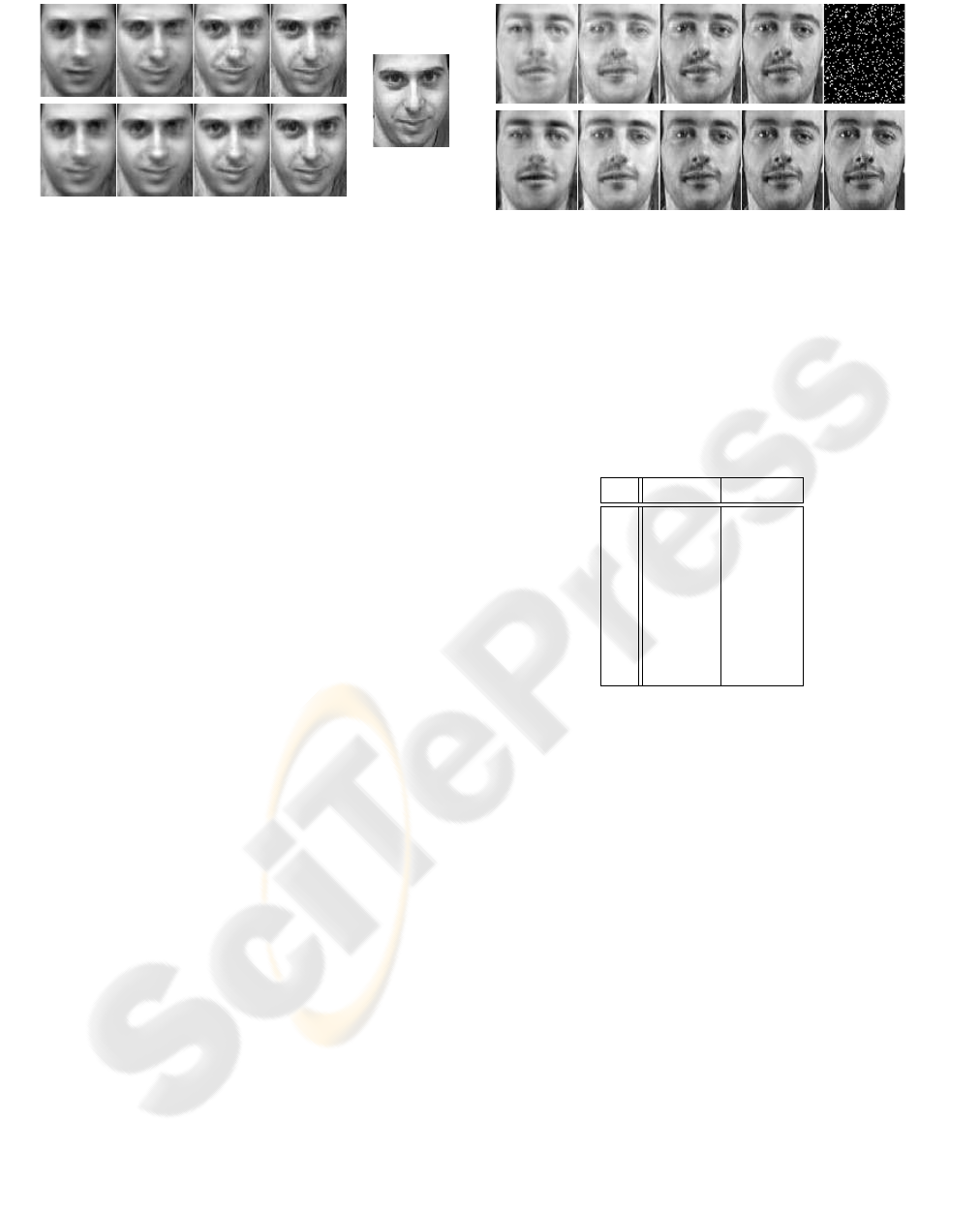
Figure 3: The reconstruction results for a familiar face. The
BPIM reconstructed images are placed at the top row for
k = 40,80, 120,160 (from left to right) and m = 2k. The
PCA reconstructed images are placed at the second row for
k = 40,80,120, 160 (from left to right). The original face is
shown on the right.
4.2 Results for Face Reconstruction
We first present in Figure 3 the reconstruction results
for a face in the training ensemble. The BPIM pro-
duces reconstructions almost as well as PCA: most
facial features captured by the PCA reconstructed im-
ages also appear in the BPIM reconstructed images.
We underline the fact that the interpolation method
requires less than 5% of the total number of pixels
N = 6660, but delivers quite satisfactory results.
To illustrate the use of the interpolation approach
for reconstructing a full image from a partial image,
we consider a face (in the training set) shown at the
bottom right and a mask shown at the top right in Fig-
ure 4. This is a relatively extreme mask that obscures
90% of the pixels in a random manner. Because the
masked face may not have intensity values at all the
best interpolation points, we need to define a new set
of interpolation points. To this end, we keep the best
interpolation points which coincide with some of the
white pixels of the masked face and replace the re-
maining best pixels with the “nearest” white pixels.
In Figure 4, the reconstructed images using those in-
terpolation points are compared with the PCA recon-
structed images utilitizing all the pixels. Although the
interpolation procedure does not recover the original
face exactly, the construction is visually close to the
“best” reconstruction.
4.3 Results for Face Recognition
We apply the face recognition system developed in
Section 3.4 to classify the probe images. We illus-
trate in Figure 5 the recognition accuracy as a function
of k for the BPIM and PCA. As it may be expected,
the BPIM yields smaller recognition rates than PCA.
However, as k increases, the BPIM gives recognition
rates which are quite comparable to those of PCA for
Figure 4: Reconstruction of a familiar face (bottom right)
from a 10% mask (top right) with only the white pixels.
The reconstructed images are shown at the top row for k =
40,80, 120, 160 (from left to right) and m = 2k. The PCA
reconstructed images are shown at the second row for k =
40,80, 120, 160 (from left to right) with using all the pixels.
Table 1: Computational times (normalized with respect to
the time to recognize a face for k = 10 and m = 20 with the
BPIM) for the BPIM and PCA at different values of k.
k
BPIM PCA
10 1.00 333.30
20 4.20 592.67
30 9.33 873.34
40 15.60 1107.66
50 26.12 1437.35
60 36.47 1708.02
70 47.93 1958.94
80 61.47 2293.73
large enough k: PCA achieves a recognition rate of
74.98%, while PBIM results in a recognition rate of
73.66% for k = 80. In many applications, the small
accuracy loss of only 1.32% is paid off very well by
the significant reduction of 6660/160(> 40) in com-
plexity. This is confirmed in Table 1 which shows
the computational times for the BPIM and PCA. The
values are normalized with respect to the time to rec-
ognize a face for k = 10 and m = 20 with the BPIM.
Clearly, the BPIM is significantly faster than PCA.
This important advantage is very useful to applica-
tions that requires a real-time recognition capability.
Finally, in order to demonstrate the classification
of incomplete images, we consider a random chosen
mask of 10% pixels shown in Figure 6. Next to the
mask, we show a few faces which are correctly rec-
ognized with using the interpolation procedure when
their intensity values are available only at the white
pixels of the mask. Note the interpolation points are
chosen in the same way as before.

0 10 20 30 40 50 60 70 80
0.3
0.35
0.4
0.45
0.5
0.55
0.6
0.65
0.7
0.75
0.8
k
RECOGNITION RATE
PCA
BPIM
Figure 5: Recognition accuracy of PCA and BPIM with in-
creasing the number of eigenfaces k. Note that the BPIM
uses m = 2k best interpolation points.
Figure 6: Recognition of incomplete face images. The 10%
mask on the left is followed by a few faces which are cor-
rectly recognized with using the interpolation procedure.
5 CONCLUSION
We have presented an interpolation method for the
reconstruction and recognition of face images. It is
important to note that PCA uses full knowledge of
the data in the reconstruction process. In contrast,
our method uses only partial knowledge of the data.
Therefore, the method is very useful to the restora-
tion of a full image from a partial image. Based
on the method, we have also developed a fully au-
tomatic real-time face recognition system. The sys-
tem is shown to be able to recognize incomplete im-
ages. Moreover, the computational cost of recogniz-
ing a new face is only O(mk), translating to a saving
of N/m relative to PCA approach. Typically, since N
is O(10
4
) and m is O(10
2
), this implies two orders of
magnitude less expensive computationally than PCA.
The significant reduction in time should enable us to
tackle very large problems. Hence, it is imperative
to test our system on a larger database such as the
FERET database. We plan to pursue this direction in
future research.
ACKNOWLEDGEMENTS
We would like to thank Professor A. T. Patera of MIT
for his long-standing collaboration and many invalu-
able contributions to this work. The authors also
thank AT&T Laboratories Cambridge for providing
the ORL face database. This work was supported by
the Singapore-MIT Alliance.
REFERENCES
Andoni, A. and Indyk, P. (2006). Near-optimal hashing al-
gorithms for approximate nearest neighbor in high di-
mensions. In Proceedings of the 47th IEEE Sym. on
Foundations of Computer Science, Berkeley, CA.
Bartlett, M. S., Movellan, J. R., and Sejnowski, T. J. (2002).
Face recognition by independent component analysis.
IEEE Trans. on Neural Networks, 13:1450–1464.
Delac, K., Grgic, M., and Grgic, S. (2005). Independent
comparative study of pca, ica, and lda on the feret
data set. International Journal of Imaging Systems
and Technology, 15(5):252–260.
Draper, B. A., Baek, K., Bartlett, M. S., and Beveridge, J. R.
(2003). Recognizing faces with pca and ica. Computer
Vision and Image Understanding, 91(1-2):115–137.
Etemad, K. and Chellappa, R. (1997). Discriminant analysis
for recognition of human face images. Journal of the
Optical Society of America A, 14(8):1724–1733.
Everson, R. and Sirovich, L. (1995). Karhunen-loeve pro-
cedure for gappy data. Opt. Soc. Am. A, 12(8):1657–
1664.
Kirby, M. and Sirovich, L. (1990). Application of the
karhunen-lo
`
eve procedure for the characterization of
human face. IEEE Transactions on Pattern Analysis
and Machine Intelligence, 12:103–108.
Lu, J., Plataniotis, K. N., and Venetsanopoulos, A. N.
(2003). Face recognition using lda-based algorithms.
IEEE Trans. on Neural Networks, 14(1):195–200.
Nguyen, N. C., Patera, A. T., and Peraire, J. (2006). A best
points interpolation method for efficient approxima-
tion of parametrized functions. International Journal
of Numerical Methods in Engineering. Submitted.
Samaria, F. S. and Harter, A. C. (1994). Parameterisation
of a stochastic model for human face identification.
In Proceedings of the 2nd IEEE workshop on Appli-
cations of Computer Vision, pages 138–142, Sarasota,
Florida.
Sirovich, L. and Kirby, M. (1987). Low-dimensional proce-
dure for the characterization of human faces. Journal
of the Optical Society of America A, 4:519–524.
Turk, M. and Pentland, A. (1991). Eigenfaces for recogni-
tion. Journal of Cognitive Neuroscience, 3(1):71–86.