
A NEW ADAPTIVE CLASSIFICATION SCHEME BASED ON
SKELETON INFORMATION
Catalina Cocianu
Dept. of Computer Science, Academy of Economic Studies, Bucharest, Romania
Calea Dorobantilor #15-17, Bucuresti –1, Romania
Luminita State
Dept. of Computer Science, University of Pitesti,Pitesti, Romania
Caderea Bastliei #45, Bucuresti – 1, Romania
Ion Roşca
Dept. of Computer Science, Academy of Economic Studies, Bucharest, Romania
Calea Dorobantilor #15-17, Bucuresti –1, Romania
Panayiotis Vlamos
Ionian University, Corfu, Greece
Keywords: Principal axes, supervised learning, pattern recognition, data mining, classification, skeleton.
Abstract: Large multivariate data sets can prove difficult to comprehend, and hardly allow the observer to figure out
the pattern structures, relationships and trends existing in samples and justifies the efforts of finding suitable
methods from extracting relevant information from data. In our approach, we consider a probabilistic class
model where each class
Hh ∈ is represented by a probability density function defined on
n
R
; where n is
the dimension of input data and H stands for a given finite set of classes. The classes are learned by the
algorithm using the information contained by samples randomly generated from them. The learning process
is based on the set of class skeletons, where the class skeleton is represented by the principal axes estimated
from data. Basically, for each new sample, the recognition algorithm classifies it in the class whose skeleton
is the “nearest” to this example. For each new sample allotted to a class, the class characteristics are re-
computed using a first order approximation technique. Experimentally derived conclusions concerning the
performance of the new proposed method are reported in the final section of the paper.
1 INTRODUCTION
Large multivariate data sets can prove difficult to
comprehend, and hardly allow the observer to figure
out the pattern structures, relationships and trends
existing in samples. Consequently, it is useful to find
out appropriate methods to summarize and extract
relevant information from data. This is becoming
increasingly important due to the size possibly
excessive large of high dimensional data.
Several authors refer to unsupervised
classification or data clustering as being the process
of investigating the relationships within data in order
to establish whether or not it is possible to compress
the information that is to validly summarize it in
terms of a relatively small number of classes
comprising similar objects in some sense (Gordon,
1999). In such a case, the whole collection given by
such a cluster can be represented by a small number
of class prototypes.
The word ‘classification’ is also used to define
the assignment process of objects to one of a set of
given classes. Thus, in pattern recognition or
discriminant analysis (Ripley, 1996; Hastie,
85
Cocianu C., State L., Ro ¸sca I. and Vlamos P. (2007).
A NEW ADAPTIVE CLASSIFICATION SCHEME BASED ON SKELETON INFORMATION.
In Proceedings of the Second International Conference on Signal Processing and Multimedia Applications, pages 85-92
DOI: 10.5220/0002137900850092
Copyright
c
SciTePress

Tibshirani &al, 2001) each object is assumed to
come from one of a known set of classes, the
problem being to infer the true class for each data.
The test performed on data are based on a finite
feature set determined either by mathematical
techniques or empirically using a training set
containing data whose true classifications are
known.
During the past decade the classification and
assignment procedures have both found a large
series of applications related to information
extraction from large size data sets, this field being
referred as data mining and knowledge discovery in
databases. (Fayyad&al, 1996; Hastie, Tibshirani
&al, 2001)
Since similarity plays a key role for both
clustering and classification purposes, the problem
of finding a relevant indicators to measure the
similarity between two patterns drawn from the
same feature space became of major importance.
The most popular ways to express the
similarity/dissimilarity between two objects involve
distance measures on the feature space. (Jain, Murty,
Flynn, 1999). In case of high dimensional data, the
computation complexity could become prohibitive,
consequently the use of simplified schemes based on
principal components, respectively principal
coordinates, provides good approximations. (Chae,
Warde, 2006) Recently, alternative methods as
discriminant common vectors, neighborhood
components analysis and Laplacianfaces have been
proposed allowing the learning of linear projection
matrices for dimensionality reduction. (Liu, Chen,
2006; Goldberger, Roweis, Hinton, Salakhutdinov,
2004)
2 DISCRIMINANT ANALYSIS
There are several different ways in which linear
decision boundaries among classes can be stated. A
direct approach is to explicitly model the boundaries
between the classes as linear. For a two-class
problem in a n-dimensional input space, this
amounts to modeling the decision boundary as a
hyperplane that is a normal vector an a cut point.
One of the methods that explicitly looks for
separating hyperplanes is the well known perceptron
model of Rosenblatt (1958), that yielded to an
algorithm that finds a separating hyperplane in the
training data if one exists.
Another method, due to Vapnik (1996) finds an
optimally separating hyperplane if one exists, else
finds a hyperplane that minimizes some measures of
overlap in the training data.
In the particular case of linearly separable
classes, in discriminating between two classes, the
optimal separating hyperplane separates and
maximizes a distance to the closest point from either
class. Not only does this provide an unique solution
to the separating hyperplane problem, but by
maximizing the margin between the two classes on
the training data this leads to better classification
performance on test data and generalization
capacities.
When the data are not separable, there will be
now feasible solutions to this problem, and
alternative formulation is needed. The disadvantage
of enlarging the space using basis transformations is
that an artificial separation through over-fitting
usually results. A more attractive alternative seems
to be the support vector machine (SVM) approach,
which allows for overlap but minimizes a measures
of the extent of this overlap.
The basis expansion method represents the most
popular technique for moving beyond linearity. It is
based on the idea of augmenting/replacing the vector
of inputs with additional variables which are
transformations of it and the use of linear models in
the augmented new space of derived input features.
The use of the basis expansions allows the
achievement of more flexible representations of
data. Polynomials, also there are limited by their
global nature, piecewise-polynomials and splines
that allow for local polynomial representations,
wavelet basis, especially useful for modeling signals
and images are just few examples of sets of basis
functions. All of them produce a dictionary
consisting of typically a very large number of basis
functions, far more than one can afford to fit to data.
Along with the dictionary, a method is required for
controlling the complexity of the model using basis
functions from the dictionary. Some of the most
popular approaches are restriction methods, where
we decide before-hand to limit the class of functions,
selections methods, which adaptively scan the
dictionary and include only those basis functions
that contribute significantly to the fit of the model
and regularization methods (as, for instance, Ridge
regression), where the entire dictionary is used but
restrict the coefficients.
Support Vector Machines (SV) are an algorithm
introduced by Vapnik and coworkers theoretically
motivated by VC theory. (Cortes, Vapnik, 1995;
Friess, Cristianini & al., 1998) SVM algorithm
works by mapping training data for classification
tasks into a higher dimensional feature space. In this
SIGMAP 2007 - International Conference on Signal Processing and Multimedia Applications
86

new feature space the algorithm looks for a maximal
margin hyperplane which separates the data. This
hyperplane is usually found using a quadratic
programming routine which is computationally
intensive, and it is non trivial to implement. SVM
have a proven impressive performance on a number
of real world problems such as optical character
recognition and face detection. However, their
uptake has been limited in practice because of the
mentioned problems with the current training
algorithms. (Cortes, Vapnik, 1995; Friess,
Cristianini & al., 1998)
The support vector machine classifier is an
extension of this idea, where the dimension of the
enlarged space is allowed to get very large, infinite
in some cases. (Hastie, Tibshirani &al, 2001)
3 PRINCIPAL DIRECTIONS -
BASED ALGORITHM FOR
CLASSIFICATION PURPOSES
The developments are performed in the framework
of a probabilistic class model where each class
Hh ∈ is represented by a probability density
function defined on
n
R
; where n is the dimension
of input data and H stands for a given finite set of
classes. The classes are learned by the algorithm
using the information contained by samples
randomly generated from them. The learning process
is based on the set of class skeletons, where the class
skeleton is represented by the principal axes
estimated from data. Basically, for each new sample,
the recognition algorithm classifies it in the class
whose skeleton is the “nearest” to this example.
(State, Cocianu 2006).
Let X be a n-dimensional random vector and let
X(1), X(2),… ,X(N), be a Bernoullian sample on X .
We assume that the distribution of X is unknown,
except the first and second order statistics. More
generally, when this information is missing, the first
and second order statistics are estimated from the
samples.
Let Z be the centered version of X, Z = X -
E(X). Let
n
WWW ,...,,
21
be a set of linear
independent vectors and
()
n
WWWW ,...,,
21
= . We
denote by
ZW
T
mm
y =
, nm ≤≤1 . The principal
axes of the distribution of X are
n
ψψψ ,...,,
2
such
that
()
m
T
mm
m
n
m
y SWW
W
RW
sup
1
2
E
=
∈
=
(1)
where S is the covariance matrix of Z.
According to the celebrated Karhunen-Loeve
theorem, the solution of (1) are unitary eigen vectors
of S,
n
ψψψ ,...,,
2
, corresponding to the eigen
values
n
λ
λ
λ
≥≥≥ ...
21
.
Once a new sample is allotted to a class, the class
characteristics (the covariance matrix and the
principal axes) are modified accordingly using first
order approximations of the new set of principal
axes. In order to compensate the effect of the
cumulative errors coming from the first order
approximations, following to the classification of
each block of
PN samples, the class skeletons are re-
computed using an exact method.
Let
N
XXX ,...,,
21
be a sample from a certain
class
C. The sample covariance matrix is
()()
∑
=
−−
−
=Σ
N
i
T
NiNiN
XX
N
1
ˆˆ
1
1
ˆ
μμ
, (2)
where
∑
=
=
N
i
iN
X
N
1
1
ˆ
μ
.
We denote by
N
n
NN
λλλ
≥≥≥ ...
21
the eigen
values and by
N
n
N
ψψ
,...,
1
a set of orthonormal eigen
vectors of
N
Σ
ˆ
.
If
X
N+1
is a new sample, then, for the series
121
,,...,,
+NN
XXXX , we get
()()
−−−
+
+Σ=Σ
+++
T
NNNNNN
XX
N
μμ
ˆˆ
1
1
ˆˆ
111
N
N
Σ−
ˆ
1
(3)
Lemma
. In case the eigen values of
N
Σ
ˆ
are
pairwise distinct, the following first order
approximations hold,
(
)()
N
iN
T
N
i
N
iN
T
N
i
N
i
N
i
ψΣψψΣψ
1
1
ˆˆ
+
+
=Δ+=
λλ
(4)
(
)
∑
≠
=
+
−
Δ
+=
n
ij
j
N
j
N
j
N
i
N
iN
T
j
N
N
i
N
i
1
1
ˆ
ψ
ψΣψ
ψψ
λλ
(5)
Proof
See (State, Cocianu , 2006 ).
The basis of the learning scheme can be described as
follows (State, Cocianu , 2006). The skeleton of C is
represented by the set of estimated principal axes
N
n
N
ψψ
,...,
1
When the example X
N+1
is included in C, then the
new skeleton is
11
1
,...,
++ N
n
N
ψψ
.
The skeleton disturbance induced by the decision
that X
N+1
has to be alloted to C is measured by
(
)
∑
=
+
=
n
k
N
k
N
k
d
n
D
1
1
,
1
ψψ
(6)
A NEW ADAPTIVE CLASSIFICATION SCHEME BASED ON SKELETON INFORMATION
87

The classification procedure identifies for each
example the nearest cluster in terms of the measure
(6). Let
{}
M
CCCH ,...,,
21
= . In order to protect
against misclassifications due to insufficient
“closeness” to any cluster, a threshold T>0 is
imposed, that is the example X
N+1
is alloted to one of
C
j
for which
()
==
∑
=
+
n
k
N
jk
N
jk
d
n
D
1
1
,,
,
1
ψψ
()
∑
=
+
≤≤
=
n
k
N
pk
N
pk
Mp
d
n
1
1
,,
1
,
1
min
ψψ
(7)
and D<T, where the skeleton of C
j
is
N
jn
N
j ,,1
,...,
ψψ
.
The classification of samples for which the
resulted value of D is larger than T is postponed and
the samples are kept in a new possible class CR. The
reclassification of elements of CR is then performed
followed by the decision concerning to either
reconfigure the class system or to add CR as a new
class in H.
For each new sample allotted to a class, the class
characteristics (the covariance matrix and the
principal axes) are re-computed using (5) and (6).
The skeleton of each class is computed using an
exact method,
M, in case PN samples have been
already classified in
{}
M
CCCH ,...,,
21
= . The
adaptive classification scheme summarized as
follows.
Let
i
C , be the set of samples coming from the
th
i class, Mi ≤≤1 ;
{
}
M
CCCH ,...,,
21
=
is the set
of pre-specified classes.
Input:
{}
M
CCCH ,...,,
21
=
REPEAT
i←1
Step 1: Let X be a new sample. Classify X according
to (7)
Step 2: If
Mi ≤≤∃1 such that X is allotted to
i
C ,
then
2.1.re-compute the characteristics of
i
C using (3), (4)
and (5)
2.2. i++
Step 3: If i<PN goto Step 1
Else
3.1. For i=
M,1 , compute the characteristics of
class
i
C using M. 3.2. goto Step 1.
UNTIL THE LAST NEW SAMPLE HAS BEEN
CLASSIFIED
Output: The new set
{}
CRCCC
M
∪,...,,
21
4 EXPERIMENTAL ANALYSIS
A series of tests were performed on bidimensional
simulated data coming from 4 clases. We use a
probabilistic model, each class being represented by
a normal density function. The closeness between
each pair of classes is measured by the Mahalanobis
distance. The estimation of the principal directions is
based exclusively on data.
The classification criterion is: allote X
N+1
to
i
j
C if
()
==
∑
=
+
i
j
ii
i
m
k
k
Nj
k
j
j
d
m
D
1
1,
,
1
ψψ
()
∑
=
+
≤≤
=
l
j
ll
l
m
k
k
Nj
k
j
j
tl
d
m
1
1,
1
,
1
min
ψψ
(8)
Because the size of the initial sample is relatively
small, we used small values of PN to compensate the
effect of the cumulative errors coming from the first
order approximations. Once a sufficient number of
new simulated examples correctly classified,
increasing values of PN are considered next.
The aims in performed tests were twofold. On
one hand it was aimed to point out the effects on the
performance of global/local closeness of the system
of classes and, on the other hand, the effects of the
geometric configurations of the principal directions
corresponding to the given classes. Some of the
results are presented in the following.
Test 1. In case the system of classes consists in four
classes, for each
41
≤
≤
i , the class
i
C ~
()
ii
N Σμ , ,
41
≤
≤
i , where
1
μ = [10 -12],
=
1
Σ
⎥
⎦
⎤
⎢
⎣
⎡
2.50 1.65
1.65 3.49
2
μ = [1 1],
=
2
Σ
⎥
⎦
⎤
⎢
⎣
⎡
6.8066 5.6105
5.6105 6.6841
3
μ = [-10 0],
=
3
Σ
⎥
⎦
⎤
⎢
⎣
⎡
2.50 1.35
1.35 1.69
4
μ = [-8 24],
=
4
Σ
⎥
⎦
⎤
⎢
⎣
⎡
12.2789 1.02
1.02 6.2789
We assume that the initial sample contains 200
examples coming from each class.
SIGMAP 2007 - International Conference on Signal Processing and Multimedia Applications
88
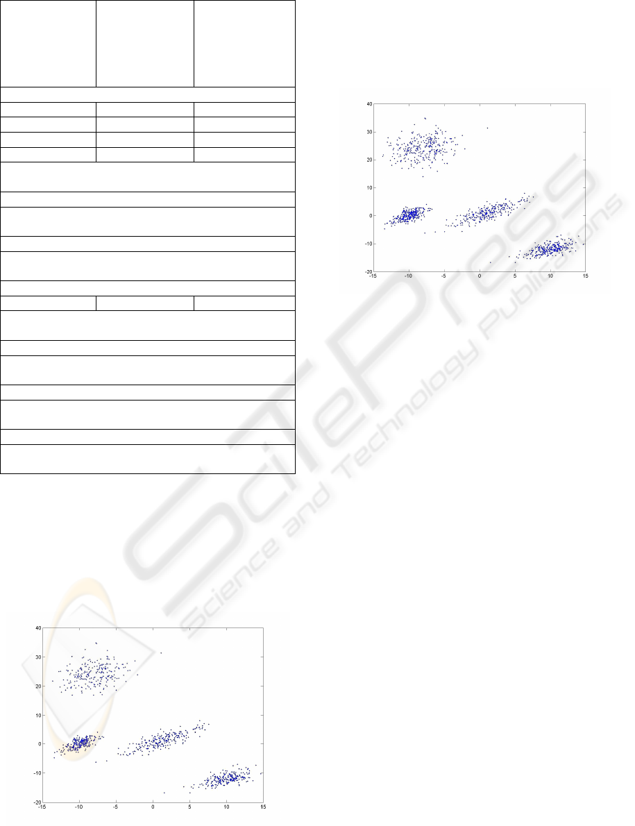
Table 1: Results on new simulated samples.
The index of
the sample in
the test set
The
misclassificatio
s
(the correct
class → the
alloted class)
Misclassified
examples
The first test set containing 20 new examples (PN=20)
2 3→2 (-7.02, 1.9)
5 4→2 (-10.06, 16.90)
14 3→2 (-7.11, 2.61)
20 4→2 (-6.38, 20.76)
4 misclassifications. For each class, compute the exact
values of its characteristics
The second test set containing 20 new examples
No misclassification. For each class, compute the exact
values of its characteristics
The third test set containing 50 new examples (PN=50)
No misclassification. For each class, compute the exact
values of its characteristics
The fourth test set containing 50 new examples
23 4→2 (-5.99, 15.88)
1 misclassified example. For each class, compute the
exact values of its characteristics
The fifth test set containing 50 new examples
No misclassification. For each class, compute the exact
values of its characteristics
The sixth test set containing 50 new examples
No misclassification. For each class, compute the exact
values of its characteristics
The seventh test set containing 50 new examples
No misclassification. For each class, compute the exact
values of its characteristics
The Mahalanobis distances between classes are
given by the entries of the matrix
⎥
⎥
⎥
⎥
⎦
⎤
⎢
⎢
⎢
⎢
⎣
⎡
0 39.4249 54.7989 152.3496
39.4249 0 33.2818 247.6876
54.7989 33.2818 0 99.4061
152.3496 247.6876 99.4061 0
.
Figure 1: The initial sample.
Note that in this example the system of classes is
relatively well separated. The tests on the
generalization capacities yielded the results
presented in table 1.
The initial sample is depicted in Figure 1. The
clusters resulted at the end of the tests are depicted
in Figure 2.
Figure 2: The clusters resulted at the end of the tests.
Test 2. In case the system of classes consists in four
classes, for each
41
≤
≤
i , the class
i
C ~
()
ii
N Σμ , ,
41
≤
≤
i , where
1
μ = [10 -12],
=
1
Σ
⎥
⎦
⎤
⎢
⎣
⎡
2.50 1.65
1.65 3.49
2
μ = [1 10],
=
2
Σ
⎥
⎦
⎤
⎢
⎣
⎡
6.8066 5.6105
5.6105 6.6841
3
μ = [-10 0],
=
3
Σ
⎥
⎦
⎤
⎢
⎣
⎡
2.50 1.35
1.35 1.69
4
μ = [-8 4],
=
4
Σ
⎥
⎦
⎤
⎢
⎣
⎡
12.2789 1.02
1.02 6.2789
We assume that the initial sample contains 200
examples coming from each class.
The Mahalanobis distances between classes are
given by the entries of the matrix
⎥
⎥
⎥
⎥
⎦
⎤
⎢
⎢
⎢
⎢
⎣
⎡
0 1.3258 6.3728 64.3167
1.3258 0 14.6578 247.6876
6.3728 14.6578 0 203.7877
64.3167 247.6876 203.7877 0
.
Note that the system of classes is such that C
2
,
C
3
, C
4
are pretty “close” and C
1
is well separated
from the others. As it is expected, the
misclassifications occur mainly for samples coming
from C
2
,
C
3
, C
4
.
A NEW ADAPTIVE CLASSIFICATION SCHEME BASED ON SKELETON INFORMATION
89

The initial sample is depicted in Figure 3 and the
clusters resulted at the end of the classification steps
are presented in Figure 4.
The closest classes in the sense of Mahalanobis
distance are C
3
and C
4
. Note that correlations of the
components are almost the same in C
3
and C
4
, but
the variability along each of the axes are
considerably larger in case of C
4
than C
3
.
In order to evaluate the capacities of our method
we tested its classification performance in
discriminating between C
3
and C
4
against the
classical discriminant algorithm. The Kolmogorov-
Smirnoff and MANOVA tests were applied to each
test set in order to derived statistical conclusions
about the closeness degree of the set of misclassified
sample and each of the classes C
3
, C
4
.
Figure 3: The initial sample.
The tests were performed on several randomly
generated samples of size 1000.
Some of the results obtained on samples coming
from C
3
and classified in C
4
are summarized in
Table 2. The entries of the table have the following
meaning. Each column corresponds to a test set. The
row entries are:
¾ the number of misclassified examples in case of
our method;
¾ the number of misclassified examples by
classical discriminant analysis method (CDA);
¾ the number of examples misclassified by our
method and misclassified by CDA;
¾ the results of Kolmogorov-Smirnoff test applied
for the group of misclassified examples against
the class identified by our classification
procedure.
¾ the results of Kolmogorov-Smirnoff test applied
for the group of misclassified examples against
the true class;
¾ the results of MANOVA applied for the group
of misclassified examples against the class
identified;
¾ the results of MANOVA applied for the group
of misclassified examples against the true class.
Figure 4: The clusters resulted at the end of the
classification steps
.
Each component of the results obtained by
Kolmogorov-Smirnoff test is either 0 or 1 indicating
for each coordinate the acceptance/rejection of the
null hypothesis using only this variable.
The test was applied on the transformed
examples such that the variables are decorrelated
using the features extracted from the misclassified
samples. The information computed by MANOVA
is summarized by retaining two indicators; the
former is either 0 or 1 and represents non-
rejection/rejection of the hypothesis that the means
are the same, but non rejection of the hypothesis
they lie on a line, the latter being the value of
Mahalanobis distance between the considered
groups.
Table 2: Some of the results obtained on samples coming
from C
3
and classified in C
4
.
Note that the performances proved by our
method are far better as compared to the classical
discriminant analysis in this case. Similar results
were obtained in a long series of tests performed in
76 67 65 76 78
132 116 122 135 132
76 67 65 76 78
1,1 1,1 1,1 1,1 1,1
0,1 0,1 0,1 0,1 1,1
0
0.095
0
0.101
1
0.125
1
0.105
0
0.095
1
4.50
1
4.199
1
3.898
1
4.408
1
4.790
SIGMAP 2007 - International Conference on Signal Processing and Multimedia Applications
90

discriminating between two classes almost
undistinguishable, where the variability in the
second class (in our case C
4
) is significant larger
than in the first class (in our case C
3
).
In Table 3 and Table 4 are summarized the
results obtained in applying the same method to the
samples coming from C
4
and misclassified in C
3
.
The entries of the Table 3 and Table 4 have the same
meaning as in Table 2.
In this case, our method and the classical
discriminant analysis method have close behaviors.
Table 3: Some of the results obtained on samples coming
from C
4
and misclassified in C
3
.
208 213 185 231 207
246 248 217 275 248
206 210 181 230 206
1,0 1,0 1,0 1,0 1,0
0,1 0,1 0,1 0,1 0,1
1
0.147
1
0.163
1
0.242
1
0.132
1
0.202
1
2.792
1
2.64
1
2.461
1
3.001
1
2.697
Table 4: Some of the results obtained on samples coming
from C
4
and misclassified in C
3
.
328 293 334 317 319
266 256 276 264 271
258 244 266 253 264
1,0 1,0 1,0 1,0 1,0
0,1 0,1 0,1 0,1 0,1
1
0.349
1
0.175
1
0.228
1
0.2932
1
0.232
1
2.616
1
2.555
1
2.624
1
2.435
1
2.577
Test 3
. The system of classes is well separated
and principal directions are pairwise orthogonal. For
each
41 ≤≤ i , the class
i
C ~
()
ii
N Σμ , , 41
≤
≤
i ,
where
1
μ = [1 19], =
1
Σ
⎥
⎦
⎤
⎢
⎣
⎡
2.5000 1.6500
1.6500 3.4900
2
μ = [4 8], =
2
Σ
⎥
⎦
⎤
⎢
⎣
⎡
=
−
0.5814 0.2749-
0.2749- 0.4165
1
1
Σ
3
μ = [-7 3], =
3
Σ
⎥
⎦
⎤
⎢
⎣
⎡
2.5000 1.3500
1.3500 1.6900
4
μ = [11 -12], =
4
Σ
⎥
⎦
⎤
⎢
⎣
⎡
=
−
0.7034 0.5619-
0.5619- 1.0406
1
3
Σ
We assume that the initial sample contains 200
examples coming from each class.
The Mahalanobis distances between classes are
given by the entries of the matrix
⎥
⎥
⎥
⎥
⎦
⎤
⎢
⎢
⎢
⎢
⎣
⎡
0 255.7000 112.8035 378.9131
255.7000 0 86.7399 45.2959
112.8035 86.7399 0 142.1112
378.9131 45.2959 142.1112 0
.
We used the values PN=50 for the first 2 steps
and PN=100 for the next steps. The performed tests
reported no misclassification.
The initial sample is depicted in Figure 5 and the
clusters resulted at the end of for classification steps
are presented in Figure 6.
Figure 5: The initial sample.
Figure 6: The clusters resulted at the end of the
classification procedure.
REFERENCES
Cortes, C., Vapnik, V., 1995. Support Vector networks. In
Machine Learning 20: 273-297
Diamantaras, K.I., Kung, S.Y., 1996. Principal
Component Neural Networks: theory and applications,
John Wiley &Sons
A NEW ADAPTIVE CLASSIFICATION SCHEME BASED ON SKELETON INFORMATION
91

Everitt, B. S., 1978. Graphical Techniques for
Multivariate Data, North Holland, NY
Fayyad, U.M., Piatetsky-Shapiro, G., Smyth, P., and
Uthurusamy, R., 1996. Advances in Knowledge
Discovery and Data Mining, AAAI Press/MIT Press,
Menlo Park, CA.
Frieß, T., Cristianini, N., and Campbell, C., 1998. The
kernel adatron algorithm: A fast and simple learning
procedure for support vector machines. In 15th Intl.
Conf. Machine Learning. Morgan Kaufmann
Publishers
Goldberger, J., Roweis, S., Hinton, G., Salakhutdinov, R.,
2004. Neighbourhood Component Analysis. In
Proceedings of the Conference on Advances in Neural
Information Processing Systems
Gordon, A.D. 1999. Classification, Chapman&Hall/CRC,
2
nd
Edition
Hastie, T., Tibshirani, R., Friedman, J. 2001. The Elements
of Statistical Learning Data Mining, Inference, and
Prediction. Springer-Verlag
Hyvarinen, A., Karhunen, J., Oja, E., 2001. Independent
Component Analysis, John Wiley &Sons
Jain,A.K., Dubes,R., 1988. Algorithms for Clustering
Data, Prentice Hall,Englewood Cliffs, NJ.
Jain, A.K., Murty, M.N., Flynn, P.J. 1999. Data clustering:
a review. ACM Computing Surveys, Vol. 31, No. 3,
September 1999
Krishnapuram, R., Keller,J.M., 1993. A possibilistic
approach to clustering. IEEE Trans. Fuzzy Syst., 1(2)
Liu, J., and Chen, S. 2006. Discriminant common vectors
versus neighbourhood components analysis and
Laplacianfaces: A comparative study in small sample
size problem. Image and Vision Computing 24 (2006)
249-262
Panayirci,E., Dubes,R.C., 1983. A test for
multidimensional clustering tendency. Pattern
Recognition,16, 433-444
Smith,S.P., Jain,A.K., 1984. Testing for uniformity in
multidimensional data, In IEEE Trans.`Patt. Anal.`
and Machine Intell., 6(1),73-81
State, L., Cocianu, C., Vlamos, P, Stefanescu, V., 2006.
PCA-Based Data Mining Probabilistic and Fuzzy
Approaches with Applications in Pattern Recognition.
In Proceedings of ICSOFT 2006, Portugal, pp. 55-60.
Ripley, B.D. 1996. Pattern Recognition and Neural
Networks, Cambridge University Press, Cambridge
.
SIGMAP 2007 - International Conference on Signal Processing and Multimedia Applications
92
