
THE ACCURACY OF SCENE RECONSTRUCTION FROM IR
IMAGES BASED ON KNOWN CAMERA POSITIONS
An Evaluation with the Aid of LiDAR Data
Stefan Lang, Marcus Hebel and Michael Kirchhof
FGAN-FOM Research Institute for Optronics and Pattern Recognition, Gutleuthausstr. 1, D-76275 Ettlingen, Germany
Keywords:
Infrared, LiDAR, evaluation, structure from motion, sensor data fusion.
Abstract:
A novel approach for the evaluation of a 3D scene reconstruction based on LiDAR data is presented. A
system for structure computation from aerial infrared imagery is described which uses known pose and position
information of the sensor. Detected 2D image features are tracked and triangulated afterwards. Each estimated
3D point is assessed by means of its covariance matrix which is associated with the respective uncertainty.
Finally a non-linear optimization (Gauss-Newton iteration) of 3D points yields the resulting point cloud.
The obtained results are evaluated with the aid of LiDAR data. For that purpose we quantify the error of a
reconstructed scene by means of a 3D point cloud acquired by a laser scanner. The evaluation procedure takes
into account that the main uncertainty of a Structure from Motion (SfM) system is in direction of the line of
sight. Results of both the SfM system and the evaluation are presented.
1 INTRODUCTION
Structure from Motion (SfM) is still an important is-
sue in Computer Vision. Over the past years there
has been done a lot of work in this area and sophisti-
cated algorithms have been developed for many appli-
cations. In case of an airborne system, as considered
in this work, the extracted 3D information can for ex-
ample be used for modelling buildings, for detecting
and tracking vehicles or for supporting the navigation.
However in case of both free motion and a fast mov-
ing sensor like a camera mounted on a helicopter, new
problems emerge because of motion blur. Addition-
ally, if an infrared sensor is used, the acquired images
contain much more noise and are of lower resolution
compared to video images.
In this paper a newly developed system for auto-
matic reconstruction of a scene from aerial infrared
imagery is described. For more accuracy in the recon-
struction and to overcome the drawbacks of feature
tracking in IR images, pose information measured by
an IMU (Inertial Measurement Unit) are used.
Normally reconstruction results of SfM systems
given as point cloud as well as dense reconstructed
models look very impressive but no quantitative mea-
sures of their correctness are available. One of the
main contribution of our work is the novel approach
to the evaluation of the scene reconstruction with the
aid of a LiDAR (Light Detecting And Ranging) sys-
tem, taking into account that the main uncertainty of
an SfM system is in direction of the line of sight. The
laser scanner employed provides very precise range
data of the scene, which are well suited as basis for
the evaluation of our SfM system. Both the IR sensor
and the laser scanner use the same INS (Inertial Nav-
igation System) and therefore have the same motion
errors. The main error is called ”drift” which occurs
because of dead reckoning. However, the laser scan-
ner can be used as ground truth for the assessment
of the SfM system anyway if no absolute evaluation
is needed. That is the case for our evaluation of the
accuracy of an SfM system with known motion infor-
mation.
The rest of this paper is organized as follows. An
overview of related work is given in section 2. In sec-
tion 3 the sensors used are briefly described. The de-
veloped algorithms and details of the SfM system are
presented in section 4. As main part of this paper,
section 5 describes the evaluation in depth. Section 6
closes the paper with a summary and future work.
2 RELATED WORK
This section is divided into two parts according to
the structure of this paper. First, existing systems
for scene reconstruction are described in relation to
439
Lang S., Hebel M. and Kirchhof M. (2008).
THE ACCURACY OF SCENE RECONSTRUCTION FROM IR IMAGES BASED ON KNOWN CAMERA POSITIONS - An Evaluation with the Aid of
LiDAR Data.
In Proceedings of the Third International Conference on Computer Vision Theory and Applications, pages 439-446
DOI: 10.5220/0001074404390446
Copyright
c
SciTePress

our system. Second, registration and evaluation algo-
rithms for 3D point clouds as well as the alignment of
2D images onto range information acquired by a Li-
DAR system are examined.
In the field of Structure from Motion there are
many different approaches to reconstruct a scene from
a given video sequence. Nist
´
er (2001) describes a sys-
tem which processes the whole chain from images
taken by an uncalibrated camera to a dense recon-
struction of the scene.
An advanced system, working with multiple cam-
eras mounted on a ground vehicle is presented in (Ak-
barzadeh et al., 2006). An urban scene is recon-
structed from long video sequences of high resolu-
tion. The collected GPS and IMU data are only used
to geo-register the reconstructed models. Their sys-
tem is divided into two parts. The first part works
online and generates a sparse 3D point cloud. In the
second part the computational expensive dense recon-
struction for the whole video sequence is performed.
In (Nist
´
er et al., 2006) visual odometry is com-
pared to pose and position estimation based on DGPS
(Differential GPS) and IMU measures. It is shown
that it is possible to use ego motion estimated from
video for an accurate image based navigation. But –
as in the other systems described above – video im-
ages of high resolution are used instead of IR images
as considered in our work.
To evaluate an extracted 3D point cloud there are
several different possibilities. A very good survey of
the field of registration and fusion of point clouds is
given in (Rodrigues et al., 2002).
For the registration of point clouds ICP (Itera-
tive Closest Point), as introduced by Besl and McKay
(1992), has been established as standard approach.
However in the case of one dense and one sparse point
cloud as in our case, the standard algorithm has to
be adjusted. In (Pottmann et al., 2004) an approach
is suggested in which a point cloud is aligned to a
surface. They introduce an alternative concept to the
ICP algorithm which relies on local quadratic approx-
imants to the squared distance function of the surface.
Alignment of video onto 3D point clouds is the
topic of (Zhao et al., 2005). They propose a method to
align a point cloud extracted from video onto a point
cloud obtained by a 3D sensor like a laser scanner.
After that a 3D model of the scene is built, which dif-
fers from our objective to perform an evaluation.
3 EXPERIMENTAL SETUP
As sensor platform a helicopter is used. The different
sensors are installed in a pivot-mounted sensor car-
rier on the right side of the helicopter. The following
sensors are used:
IR Camera. An AIM 640QMW is used to acquire
mid-wavelength (3-5µm) infrared light. The lens
has a focal length of 28mm and a field of view of
30.7
◦
× 23.5
◦
.
LiDAR. The Riegl Laser Q560 is a 2D scanning de-
vice which illuminates in azimuth and elevation
with short laser pulses. The distance is calculated
based on the time of flight of a pulse. It covers
almost the same field of view as the IR camera.
INS. The INS (Inertial Navigation System) is an Ap-
planix POS AV system which is specially de-
signed for airborne usage. It consist of an IMU
and a GPS system. The measured pose and po-
sition are Kalman-filtered to smooth out errors in
the GPS.
The range resolution of the LiDAR system is about
0.02m according to the specifications given by the
manufacturer. The absolute accuracy specifications
of the Applanix system state the following accura-
cies (RMS): position 4-6m, velocity 0.05m/s, roll and
pitch 0.03
◦
and true heading 0.1
◦
. As described in
the introduction, both the SfM system and the LiDAR
system use the same INS and thus have the same ab-
solute position and pose error. Therefore the accuracy
of the INS is irrelevant for the comparison of both sys-
tems.
Because of the low noise of the laser system (some
centimeters) compared to the SfM system (some me-
ters) that noise will be neglected in this paper.
For the later fusion to be successful, the measured
data is registered in time first. Different frequencies
as well as the integration time of the IR camera are
taken into account.
Both the coordinate frame of the IR camera and of
the laser scanner are given in respect of the INS refer-
ence coordinate frame. Therefore coordinate transfor-
mations between the IR camera and the laser scanner
are known and later evaluation is possible.
4 3D RECONSTRUCTION
The developed system automatically calculates a set
of 3D points from given IR images, pose and position
information. For implementation Intel’s computer vi-
sion library OpenCV (Intel, 2006) is used.
A system overview is given in figure 1. After ini-
tialization, detected features are tracked image by im-
age. To minimize the number of mismatches between
the corresponding features in two consecutive images
the algorithm checks the epipolar constraint by means
VISAPP 2008 - International Conference on Computer Vision Theory and Applications
440
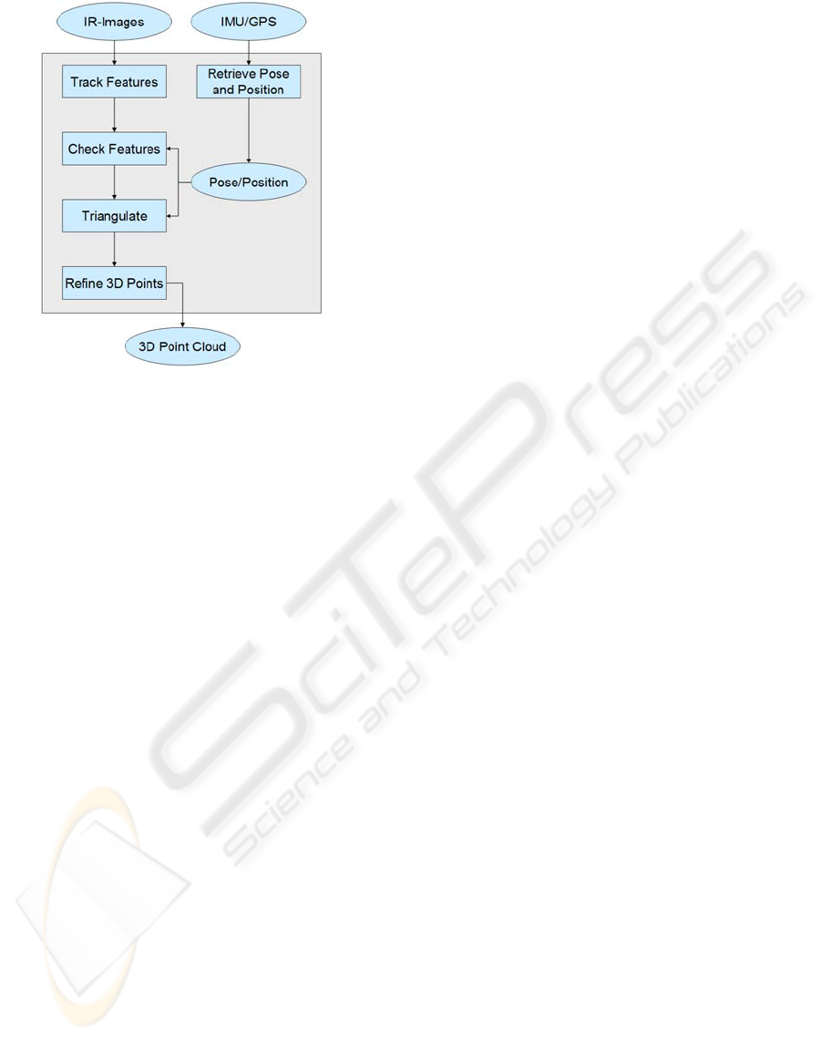
Figure 1: System overview of the modules. Features are
tracked in consecutive images and checked for satisfaction
of the epipolar constraint. Linear Triangulation of each
track of the checked features gives the 3D information. In
both steps – constraint checking and triangulation – the re-
trieved pose and position information is used. Finally each
3D point is evaluated and optimized.
of the given pose information retrieved from the INS.
Triangulation of the tracked features results in the 3D
points. Each 3D point is assessed with the aid of
its covariance matrix which is associated with the re-
spective uncertainty. Finally a non-linear optimiza-
tion yields the completed point cloud.
The modules are described in detail in the rest of
this section.
4.1 Tracking Features
To estimate the motion between two consecutive im-
ages the OpenCV version of the KLT tracker (Shi and
Tomasi, 1994) is used. This pyramidal implementa-
tion is very computational efficient and does a bet-
ter job of handling features near the image borders
than the original version. A precise description can
be found in (Bouguet, 2000).
The algorithm tracks point features such as cor-
ners or points with a neighbourhood rich in texture.
For robust tracking a measure of feature similarity is
used. This weighted correlation function quantifies
the change of a tracked feature between the current
image and the image of initialization of the feature.
4.2 Retrieve Pose and Position
The INS gives the Kalman-filtered absolute position
and pose of the reference coordinate frame. Three
angles (roll, pitch and yaw) describe the orientation in
space. The position is given in longitude and latitude
according to World Geodetic System 1984 (WGS84).
After converting the data into absolute rotation
matrices R
abs
i
and position vectors
˜
C
i
for the abso-
lute pose and position of the i-th camera in space, the
projection matrices P
i
, needed for triangulation, are
calculated as follows
P
i
= KR
abs
i
[I
3
| −
˜
C
i
], (1)
where I
3
is the unit matrix. Altogether P
i
is a 3 × 4-
matrix. The intrinsic camera matrix K is defined as
K =
f 0 −x
c
0 f −y
c
0 0 1
, (2)
with focal length f and principle point (x
c
,y
c
).
4.3 Epipolar Constraint
Let R and t be the relative rotation and translation of
the camera between two consecutive images. Further
let x be a feature in one image and x
0
be a feature in
the other image. If both features belong to the same
point X in 3-space, then the image points have to sat-
isfy the following constraint
x
0 T
Fx = 0. (3)
The fundamental matrix F is the unique (up to scale)
rank 2 homogeneous 3 × 3-matrix which satisfies the
constraint given in equation (3). To retrieve the fun-
damental matrix, as described in (Hartley and Zisser-
man, 2004), the essential matrix has to be computed
by means of the given relative orientation of the cam-
eras
E = [t]
×
R. (4)
The 3 × 3-matrix [t]
×
is the skew-symmetric matrix
of the vector t. Next, F can be calculated directly as
follows
F = K
T
−1
EK
−1
= K
T
−1
[t]
×
RK
−1
. (5)
To check if x
0
is the correct image point corresponding
to the tracked point feature x of the previous image,
x
0
has to lie on the epipolar line l
0
defined as
l
0
≡ Fx. (6)
Normally a corresponding image point doesn’t lie ex-
actly on the epipolar line, due to noise in the images
and inaccuracies in pose measures. Therefore if the
distance (error) of x
0
to l
0
is too large, the found fea-
ture is rejected and the track ends.
THE ACCURACY OF SCENE RECONSTRUCTION FROM IR IMAGES BASED ON KNOWN CAMERA POSITIONS
- An Evaluation with the Aid of LiDAR Data
441
4.4 Triangulation
During iteration over the IR images, tracks are built of
detected and tracked point features. If an image fea-
ture can’t be retrieved or doesn’t satisfy the epipolar
constraint, the track ends and the corresponding 3D
point X is calculated. In (Hartley and Sturm, 1997) a
good overview of different methods for triangulation
is given as well as a description of the method used in
our system.
Let x
1
...x
n
be the image features of the tracked
3D point X in n images and P
1
...P
n
the projection
matrices of the corresponding cameras. Each mea-
surement x
i
of the track represents the reprojection of
the same 3D point
x
i
≡ P
i
X for i = 1 . . . n. (7)
With the cross product the homogeneous scale fac-
tor of equation (7) is eliminated, which leads to
x
i
× (P
i
X) = 0. Subsequent there are two linearly
independent equations for each image point. These
equations are linear in the components of X, thus they
can be written in the form AX = 0 with
A =
x
1
p
3T
1
− p
1T
1
y
1
p
3T
1
− p
2T
1
.
.
.
x
n
p
3T
n
− p
1T
n
y
n
p
3T
n
− p
2T
n
, (8)
where p
kT
i
are the rows of P
i
. The 3D point X is the
unit singular vector corresponding to the smallest sin-
gular value of the matrix A.
4.5 Non-Linear Optimization
After triangulation the reprojection error can be esti-
mated as follows
ε
i
=
ε
x
i
ε
y
i
!
= d(X,P
i
,x
i
) =
x
i
−
p
1
i
X
p
3
i
X
y
i
−
p
2
i
X
p
3
i
X
. (9)
To calculate the covariance matrix, the Jacobian ma-
trix J, which is the partial derivative matrix ∂ε/∂X, is
needed first:
J =
∂ε
x
1
∂X
∂ε
x
1
∂Y
∂ε
x
1
∂Z
∂ε
y
1
∂X
∂ε
y
1
∂Y
∂ε
y
1
∂Z
.
.
.
∂ε
x
n
∂X
∂ε
x
n
∂Y
∂ε
x
n
∂Z
∂ε
y
n
∂X
∂ε
y
n
∂Y
∂ε
y
n
∂Z
(10)
With the assumption of a reprojection error of one
pixel, the back propagated covariance matrix of a 3D
point is calculated
Σ
X
=
J
T
J
−1
. (11)
The euclidean norm of Σ
X
gives an overall measure
of the uncertainty of the 3D point X, and enables the
algorithm to reject poor triangulation results.
With non-linear optimization, a calculated 3D
point can be corrected. Let ε(X + ξ) be the corrected
version of (9) by a vector ξ. A first order Taylor ap-
proximation yields
ε(X + ξ) ≈ ε + Jξ. (12)
Then the correction ξ can be estimated assuming
ε(X + ξ) = 0 by
ξ = −
J
T
J
−1
J
T
ε. (13)
This procedure can be repeated until the corrections
of the 3D point fall below a certain threshold. In our
case the algorithm performs only one iteration which
showed to be a reasonable optimization.
4.6 Results
We tested our system on an infrared image sequence
with 470 images with a resolution of 624 × 480. Dur-
ing the recording, the pitch angle of the sensor carrier
had been 45
◦
from the initial down looking position.
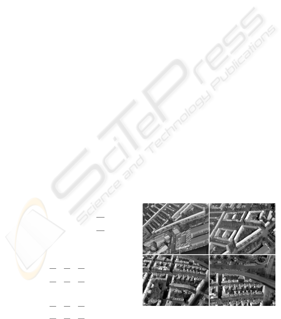
Figure 2 shows four sample images of the processed
sequence. To get a better overview of the whole se-
quence, figure 3 displays a panorama of all images.
It was generated with image to image homographies
calculated with the tracked features, see section 4.1.
Working on that sequence and taking pose and
position information into account the system calcu-
lates an optimized point cloud of about 17,500 points,
Figure 2: Four sample images of the sequence.
VISAPP 2008 - International Conference on Computer Vision Theory and Applications
442
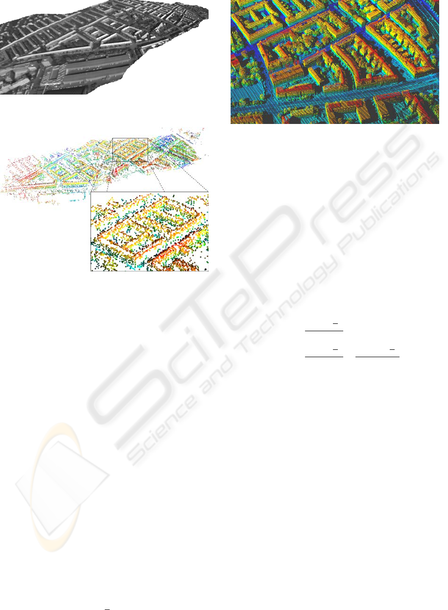
Figure 3: Panorama of the processed image sequence.
Figure 4: Calculated point cloud of the image sequence with
the magnification of one building. The overall number of
points is 17,606.
see figure 4. One building is magnified for a better
view. The height of each point is coded in its color.
Although it is a sparse reconstruction, the structure
of each building is well distinguishable and there are
only a few outliers due to the performed optimization.
5 EVALUATION WITH LIDAR
The previously presented SfM system reconstructs the
area by a sparse 3D point cloud, see figure 4. Next the
calculated result shall be evaluated quantitatively with
the aid of LiDAR data. Therefore a novel benchmark
for a SfM system by means of given 3D information
has been developed. For the evaluation an error mea-
sure for the overall accuracy of the point cloud is ob-
tained.
5.1 3D Reconstruction with LiDAR
The employed LiDAR system scans the area line-by-
line. The distance d of each 3D point to the sensor is
calculated based on the time of flight t of the emitted
light pulse as follows
d =
t
2
c
0
, (14)
Figure 5: Reconstructed area with color coded height of the
LiDAR points.
where c
0
is the speed of light. After conversion into
the reference coordinate frame an almost dense recon-
struction in form of a 3D point cloud is obtained. Fig-
ure 5 shows a cutout of the area.
Let
ˆ
d be the correct distance of a point to the cam-
era and ∆d the measuring error, then the following
relation is obtained
ˆ
d = d + ∆d. (15)
With the angle of beam ψ and count of measures κ
along a scan line, the average point spacing ∆
¯
b can be
calculated as follows:
∆
¯
b =
2
ˆ
d tan(
ψ
2
)
κ
(16)
=
2d tan(
ψ
2
)
κ
+
2∆d tan(
ψ
2
)
κ
. (17)
With the second summand of equation (17) it is also
possible to estimate the average error of the distance
between points along a scan line.
In our case the error of the used LiDAR system in
direction of the line of sight is about 0.2m at a distance
of 550m. With 1000 measures along one scan line and
an angle of beam of 60
◦
, the obtained average spacing
between points is about 0.7m. The calculated error
between points, see equation (17), is less than 1cm
and therefore this error can be neglected.
5.2 Comparison
Both point clouds have been acquired during the
same flight. Our SfM algorithm has calculated about
17,500 points. In contrast, the dense point cloud ob-
tained by the 3D scanner consists of more the 1.5 mil-
lion points. Because both 3D point clouds are geo-
referenced it is possible to superimpose the sparse
SfM point cloud to the dense LiDAR point cloud, see
figure 6.
THE ACCURACY OF SCENE RECONSTRUCTION FROM IR IMAGES BASED ON KNOWN CAMERA POSITIONS
- An Evaluation with the Aid of LiDAR Data
443
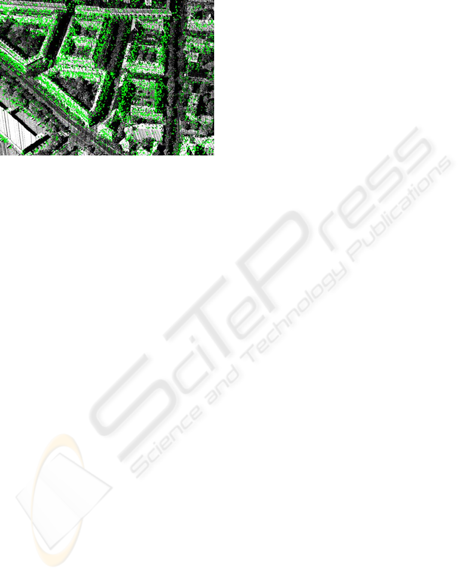
Figure 6: LiDAR point cloud with superimposed (green)
points calculated by the SfM system.
Though it is possible to superimpose one point
cloud to the other, no quantitative measure of the ac-
curacy can be obtained in this way because of the fol-
lowing reasons:
• Points of the SfM point cloud represent tracked
image features which were good to track whereas
points of the LiDAR data are almost uniformly
distributed over the observed area.
• There is a significant difference in the size of both
point clouds.
• There is a large difference especially in direction
of line of sight of both point clouds. The laser
points have a variance of approximately 0.2m
whereas the 3D points reconstructed by the SfM
system are distributed with a variance of several
meters in that direction.
Using the ICP algorithm results in a translation and
rotation of the sparse point cloud which minimize
the distances between the closest points of both point
clouds respectively. However there is no guarantee
that in each case the closest point is the actually cor-
responding point. Additionally, it is hard to obtain
a significant measure from that calculated displace-
ment.
5.3 Evaluation Approach
As described before a 3D point reconstructed from
IR images is mostly inaccurate in the line of sight.
Taking that into account as well as the other listed
issues of section 5.2 we developed a novel evaluation
approach described in the following.
For each 3D point of the SfM point cloud, the al-
gorithm iterates through the IR images in which the
considered 3D point was detected during tracking.
Then the following steps are executed:
1. Create a line through camera center and consid-
ered 3D point of the SfM point cloud
2. Find k nearest 3D points from LiDAR point cloud
to that line
3. Calculate distances of found k neighbours to con-
sidered 3D point of the SfM point cloud
In each iteration the smallest distance, calculated in
step (3), is added to a sum. For each 3D point this sum
is normalized afterwards by the number of considered
views, which yields the average error.
The following pseudo code describes the algo-
rithm more clearly and it simplifies considerations of
complexity of the program.
For i = 1..n (all SfM 3D points) do
Sum[i] = 0
For j = 1..m (all IR images) do
If 3D point is visible
(1) Calculate line through camera center
and 3D point
(2) Get k nearest 3D points of LiDAR
point cloud to that line
(2.1) dist = distance of nearest
one to considered
SfM point
(3) Sum[i] = Sum[i] + dist
End
End
Eval[i] = Sum[i]/m
End
After running the program, the i-th entry of the ar-
ray Eval is the average distance of the i-th SfM 3D
point to all of its LiDAR counterparts from consid-
ered views. As wanted the algorithm prefers LiDAR
3D points with small distances perpendicular to the
line of sight during the search for corresponding 3D
points.
With that result, we obtained an overall measure
for the accuracy of reconstructed 3D points. Consid-
eration of the complexity of our program shows the
hotspot step (2) where the k nearest 3D points of Li-
DAR data to a line are calculated. The complexity of
the algorithm is O(nmq), with n and m defined as in
the pseudo code above and q the number of LiDAR
points. Because of the negligible number of consid-
ered images m compared to the amount of points, m
can be omitted and therefore the complexity of O(nq)
is obtained.
For computational simplification the approach to
search corresponding LiDAR points to a presently
considered SfM point is changed. Instead of the iter-
ation over all LiDAR points for each 3D point of the
SfM point cloud and for each considered view, the Li-
DAR point cloud is reprojected to the view of each IR
camera. This computation is executed once and im-
ages comparable to the IR images are obtained. With
VISAPP 2008 - International Conference on Computer Vision Theory and Applications
444
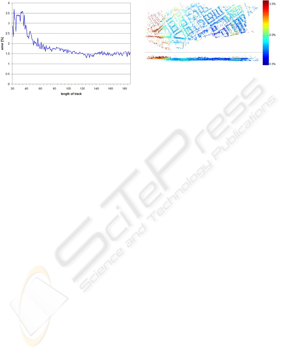
Figure 7: Relationship between the relative error to the dis-
tance to the IR camera and the length of track. With in-
creasing length of track, the accuracy of the reconstructed
3D point gets better.
that result there is a direct correspondence between a
previously tracked IR image feature and a reprojected
laser point at the same coordinates. To estimate the
corresponding laser point, all neighbours of the image
feature are taken into account. Those are the points of
the laser point cloud, which are close to the line of
sight of the currently considered view. The one with
the smallest distance to the 3D point of the SfM point
cloud is regarded as correspondence. The rest of the
program stays unchanged.
5.4 Evaluation Results
Evaluation of the reconstructed scene shows that there
are some 3D points with no corresponding LiDAR 3D
points. These points lie at the outside margin of the
considered scene where no LiDAR data is available.
However less than 500 points of total over 17,500
points are affected. Therefore an evaluation of about
17,000 points is possible.
In the following the errors of reconstructed 3D
points are given relatively to their distance to the IR
camera.
The relation of the error of a reconstructed 3D
point and the number of considered views for trian-
gulation is shown in figure 7. As expected, an image
feature tracked for a long time leads to a better esti-
mation of the corresponding 3D point than one found
in a small number of images. Errors of less than 2
percent are reached for tracks longer than 50 frames.
Overall the average error of the reconstructed scene
is about 1.8 percent. The absolute error, average dis-
tances of SfM 3D points to LiDAR 3D points, is about
10 meters at sensor-scene distances of about 550m.
This error is mainly in direction of the line of sight.
Figure 8: Color coded error of the calculated point cloud.
Blue represents a small error whereas the color red repre-
sents a high error. The scene is shown from top view (top)
and from side view (bottom).
Another presentation of the distribution of the er-
ror is given in figure 8. It shows the estimated point
cloud with color coded error. Comparably good re-
constructed points are blue whereas red points are of
lower accuracy. Noticeable is the red area on the left
side of the point cloud. There are two reasons which
explain this bad reconstructed sector. First, during ac-
quisition the helicopter flew a curve in this area which
means that there are a lot of changes between two
consecutive images. Second, the considered image
sequence started at this section. Therefore average
length of track of computed 3D points in this area is
less than in the rest of the reconstructed scene.
6 CONCLUSIONS
We have developed a system to reconstruct a scene
from an IR sequence. To overcome the drawbacks of
IR images used for feature tracking, pose information
measured by an IMU are used. For measuring the ac-
curacy of the reconstructed scene, we have presented
a novel benchmark by means of given LiDAR data.
This evaluation takes the functionality of a SfM sys-
tem into account.
In future work we will use our developed evalu-
ation method for improvements and tests of our SfM
system. Additionally we will test the accuracy of the
estimation of ego motion from IR images.
REFERENCES
Akbarzadeh, A., Frahm, J.-M., Mordohai, P., Clipp, B., En-
gels, C., Gallup, D., Merrell, P., Phelps, M., Sinha, S.,
Talton, B., Wang, L., Yang, Q., Stewenius, H., Yang,
R., Welch, G., Towles, H., Nister, D., and Pollefeys,
M. (2006). Towards urban 3d reconstruction from
video. In 3DPVT ’06: Proceedings of the Third In-
ternational Symposium on 3D Data Processing, Visu-
THE ACCURACY OF SCENE RECONSTRUCTION FROM IR IMAGES BASED ON KNOWN CAMERA POSITIONS
- An Evaluation with the Aid of LiDAR Data
445

alization, and Transmission (3DPVT’06), pages 1–8,
Washington, DC, USA. IEEE Computer Society.
Besl, P. J. and McKay, N. D. (1992). A method for regis-
tration of 3-d shapes. IEEE Transactions on Pattern
Analysis and Machine Intelligence, 14(2):239–256.
Bouguet, J.-Y. (2000). Pyramidal implementation
of the lucas kanade feature tracker. The pa-
per is included in the OpenCV distribution, see
www.intel.com/technology/computing/opencv.
Hartley, R. I. and Sturm, P. (1997). Triangulation. Computer
Vision and Image Understanding, 68(2):146–157.
Hartley, R. I. and Zisserman, A. (2004). Multiple View Ge-
ometry in Computer Vision. Cambridge University
Press, ISBN: 0521540518, second edition.
Intel (2006). Opencv - open source computer vision library.
www.intel.com/technology/computing/opencv.
Nist
´
er, D. (2001). Automatic Dense Reconstruction from
Uncalibrated Video Sequences. PhD thesis, Royal In-
stitute of Technology KTH.
Nist
´
er, D., Naroditsky, O., and Bergen, J. (2006). Visual
odometry for ground vehicle applications. Journal of
Field Robotics, 23(1).
Pottmann, H., Leopoldseder, S., and Hofer, M. (2004). Reg-
istration without icp. Computer Vision and Image Un-
derstanding, 95(1):54–71.
Rodrigues, M., Fisher, R., and Liu, Y. (2002). Special issue
on registration and fusion of range images. Computer
Vision and Image Understanding, 87(1-3):1–7.
Shi, J. and Tomasi, C. (1994). Good features to track.
In IEEE Conference on Computer Vision and Pattern
Recognition (CVPR’94), pages 593–600, Seattle.
Zhao, W., Nist
´
er, D., and Hsu, S. (2005). Alignment of
continuous video onto 3d point clouds. IEEE Trans-
actions on Pattern Analysis and Machine Intelligence,
27(8):1305–1318.
VISAPP 2008 - International Conference on Computer Vision Theory and Applications
446
