
LOCAL HISTOGRAM BASED DESCRIPTORS FOR RECOGNITION
Oskar Linde and Lars Bretzner
CVAP/CSC, KTH, Stockholm, Sweden
Keywords:
Image representation, Image descriptor, Histogram, Invariance, Categorization.
Abstract:
This paper proposes a set of new image descriptors based on local histograms of basic operators. These
descriptors are intended to serve in a first-level stage of an hierarcical representation of image structures.
For reasons of efficiency and scalability, we argue that descriptors suitable for this purpose should be able
to capture and separate invariant and variant properties. Unsupervised clustering of the image descriptors
from training data gives a visual vocabulary, which allow for compact representations. We demonstrate the
representational power of the proposed descriptors and vocabularies on image categorization tasks using well-
known datasets. We use image representations via statistics in form of global histograms of the underlying
visual words, and compare our results to earlier reported work.
1 INTRODUCTION
1.1 Background and Motivation
In this work we explore local image descriptors based
on histograms of basic operators, applied on a grid. In
previous work (Linde and Lindeberg, 2004), we have
shown how global histogram-based descriptors show
surprisingly good classification performance on well-
known image data sets; here we compare the results
with the performance of the proposed local descrip-
tors, giving a much more compact representation.
The representation is based on a dense grid struc-
ture applied on the image. Dense grid-based repre-
sentations have been claimed to better handle recogni-
tion and segmentation of a wide range of textures, ob-
jects and scenes (Lazebnik et al., 2006; Bosch et al.,
2007; Agarwal and Triggs, 2006; Jurie and Triggs,
2005), compared to representations based on sparse
local interest points (Schiele and Crowley, 2000;
Lowe, 2004; Dorkó and Schmid, 2005; Csurka et al.,
2004). One main reason is that methods relying on
interest point detectors naturally show poor recogni-
tion/classification performance in image areas where
such detectors give no or few responses. Representa-
tions including local histograms have been proposed
by e.g. (Koenderink and Doorn, 1999) and there are
many examples of histogram-based image descriptors
in the literature, both global (Schiele and Crowley,
2000; Nilsback and Caputo, 2004), and local (Lowe,
2004; Puzicha et al., 1999; Schmid, 2004). One ad-
vantage of such descriptors is that they show robust-
ness to small image perturbations, like noise, minor
occlusions, translations and distortions.
The proposed descriptors have been tested on ob-
ject classification problems present in a number of im-
age data sets frequently used for testing image classi-
fication frameworks. An unsupervised clustering of
the descriptor responses from the training set gives a
visual vocabulary. We look upon this vocabulary as
a possible building block of higher-lever, semi-local
descriptors. In this work however, in order to test the
descriptors we use the vocabulary to represent each
object class as a global histogram of words. Simi-
lar techniques have been used by e.g. (Csurka et al.,
2004; Dorkó and Schmid, 2005; Fei-Fei and Perona,
2005). The here proposed multi-scale descriptors are
rotationally invariant. We show how a contrast nor-
malization procedure makes the descriptors invariant
to contrast changes that could be caused by e.g. vary-
ing illumination, and how the normalization increases
classification performance. The presented work in-
clude comparisons to earlier similar global descrip-
tors for classification problems.
1.2 Invariant Image Descriptors
It is advantageous to separate the image data as far as
possible into independent components. This separa-
tion should be done at a low level, while still keeping
the possibility to model joint probabilities on higher
levels. When the data is as separated as possible, the
system can at a low level learn structures and features
332
Linde O. and Bretzner L. (2009).
LOCAL HISTOGRAM BASED DESCRIPTORS FOR RECOGNITION.
In Proceedings of the Fourth International Conference on Computer Vision Theory and Applications, pages 333-339
DOI: 10.5220/0001793103330339
Copyright
c
SciTePress
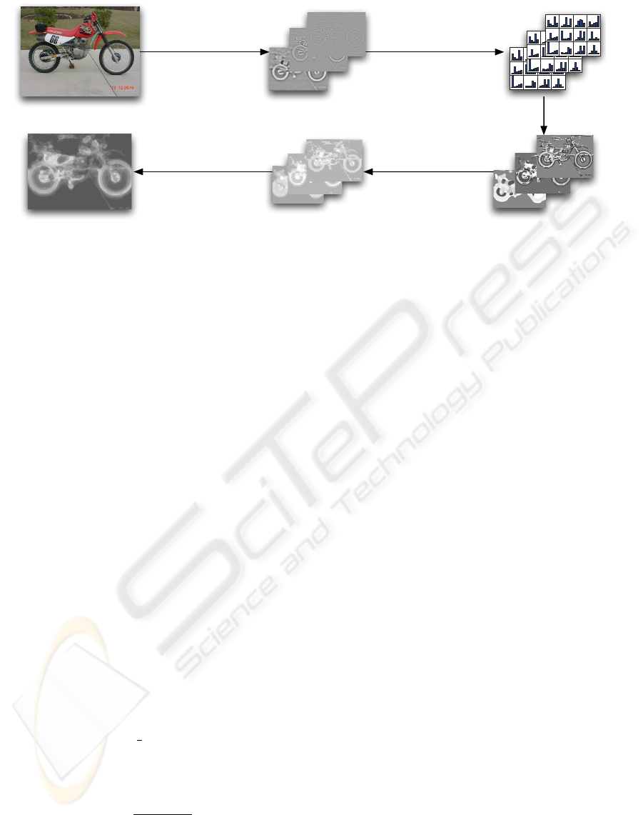
4. Class Probability
5. Probability Map
A B C
DEF
1. Image Operators
Multiple Scales
2. Normalized Histograms
Computed in Grid
3. Vocabulary
Quantization
Figure 1: Schematic representation of the system. The steps are described in section 2.
independently of other separated components. This
means that a much smaller amount of training data
is needed to learn the variations over certain sepa-
rated feature components. The joint features of the
combined components can then be learned at a higher
level, at a vastly reduced domain of data.
2 REPRESENTATION AND
MATCHING
Figure 1 shows an overview of the processing scheme
in which we use and test the proposed descriptors.
This section describes the scheme, the main part of
the paper focuses on the first three steps.
2.1 Image Operators
The local image descriptors we study in this work are
built up by the following components:
• Normalized Gaussian derivatives, obtained by
computing partial derivatives (L
x
,L
y
,L
xx
,L
xy
,L
yy
)
from the scale-space representation L(·,·; t) =
g(·,·; t) ∗ f obtained by smoothing the original
image f with a Gaussian kernel g(·,·; t), and mul-
tiplying the regular partial derivatives by the stan-
dard deviation σ =
√
t raised to the order of dif-
ferentiation (Lindeberg, 1994).
• Differential invariants, invariant to rotations in the
image plane, we use the normalized gradient mag-
nitude |∇
norm
L| =
q
t(L
2
x
+ L
2
y
), and the normal-
ized Laplacian ∇
2
norm
L = t(L
xx
+ L
yy
).
• Chromatic cues from RGB-images according to
C
1
= (R −G)/2 and C
2
= (R + G)/2 −B.
Unless otherwise mentioned, all primitives are
computed at scale levels σ ∈ {1,2,4}. For the data
sets studied in this work, this choice is reasonable, as
they do not include major scale variations.
Using these image primitives, we build the follow-
ing rotationally invariant point descriptors:
• 3-D (∇
2
L; σ = 1, 2, 4) is the Laplacian applied on
the gray level scale space image L at the scales
σ ∈ {1,2, 4}.
• 5-D (∇
2
L; σ = 1,2,4),(∇
2
C; σ = 2) is the Lapla-
cian applied on L at the scales σ ∈{1,2,4} and on
the two chromatic channels C at the scale σ = 2.
• 6-D (|∇L|, ∇
2
L; σ = 1, 2, 4) is the gradient magni-
tude |∇ ·| and the Laplacian ∇
2
·applied to L at the
scales σ ∈ {1,2, 4}
• 3-D (L,C; σ = 1) is analogous to the classic color
histogram descriptor of (Swain and Ballard, 1991)
applied to L and C at the scale σ = 1.
This selection of point descriptors have been
shown to perform well as components of global his-
togram based descriptors in previous work, see (Linde
and Lindeberg, 2004).
The different descriptors capture different ele-
ments of the image. The 3-D color histogram captures
the color distribution of an area and is invariant to any
structure within the area. The Laplacian operator, ∇L
captures structures of a certain size, corresponding to
its scale. The resulting histogram of the Laplacian op-
erator applied at different scales will capture the fre-
quency of structures, such as lines of different widths
and blobs of different sizes. The ∇
2
C operator cap-
tures the same structures in the color domain.
2.2 Local Receptive Field Histograms
The image is divided into regularly distributed and
partially overlapping local image areas. The N-D de-
LOCAL HISTOGRAM BASED DESCRIPTORS FOR RECOGNITION
333

scriptors as described in section 2.1 are applied to
each point of the area, resulting in a N-dimensional
feature vector x, at each point. The local image areas
are defined by an accumulation function with a square
shape 24×24. (A performance study comparing dif-
ferent window sizes and accumulator functions is pre-
sented in (Linde and Bretzner, 2008).) The window
size is optimized for the experimental setup in this pa-
per, smaller image regions could be more appropriate
when the descriptors are used in a feature hierarchy.
For each such local image area, a weighted local con-
trast normalization is performed. This normalization
step is further explained in section 2.3. After nor-
malization, the N-dimensional feature vectors of the
local image area are quantized and accumulated in a
q
1
×q
2
×... ×q
N
-dimensional histogram.
2.3 Contrast Normalization
Contrast normalization is important for several rea-
sons. It makes the system more robust to contrast
changes over the image caused by lighting and shad-
ows and reduces the amount of training data required
to learn and categorize the various image structures
encountered. The local contrast factor is factored
out and kept as an independent value for each sub-
window. The contrast factor could be used at a later
stage for a richer description of the image.
The normalization is applied to local regions to at-
tain invariance to local contrast variations as follows:
From a b ×b sized sub-window, N-dimensional fea-
ture vectors
{
x
1
,x
2
,...,x
b
2
}
are computed. The fea-
ture vectors are supplied by a predetermined set of
weights,
{
w
1
,w
2
,...,w
b
2
}
.
The different dimensions of the feature vector are
assigned to k normalization groups, G, so that each
normalization group, G
i
, contains a subset of dimen-
sion indices, I: G
i
=
{
I
i
1
,I
i
2
,...
}
, where 1 ≤ I
j
≤ N.
Each dimension index I
j
may belong to at most one
normalization group G
i
.
Each dimension of the feature vectors has a mean,
m
j
that is either set to 0 for dimensions corresponding
to operators whose responses are expected to be sym-
metric around 0, such as the Laplacian and normal-
ized gaussian derivatives, or computed for operators,
such as the intensity, that has no natural mid-point.
The variance for each dimension is computed:
v
j
=
b
2
∑
i=1
(x
i
j
−m
j
)
2
b
2
(1)
The variance for each normalization group is the
mean variance of its corresponding dimensions:
V
i
=
∑
j∈G
i
v
j
|
G
i
|
(2)
Each feature vector x is quantized into a vector y:
y
j∈G
i
=
0 x
j
−m
j
<−3
√
V
i
q
j
−1 3
√
V
i
≤x
j
−m
j
j
q
j
(x
j
−m
j
+3
√
V
i
)
6
√
V
i
k
−3
√
V
i
≤x
j
−m
j
<3
√
V
i
(3)
In order to avoid amplifying noise in low contrast
areas, a threshold is set from the assumed noise level
of the images. All areas with a variance below the
noise threshold are assumed to be uniform and are
therefore normalized by a zero variance, which will
result in a local histogram containing only one non-
zero bin. The effects of contrast normalization and
different levels of the noise threshold are studied in
section 3.1.
2.4 Visual Vocabulary
A visual vocabulary is formed by an unsupervised
clustering of histograms from random regions of a set
of training images. The number of clusters or words,
K, is a predefined parameter. The clustering algorithm
used is K-means with a limited number of iterations.
It is stopped at the first local minimum (which usually
happened after about 20–30 iterations for the experi-
ments in this paper). The distance metric used for the
clustering is the Bhattacharyya distance, defined as:
d(h,t) =
r
1 −
∑
i
p
h(i) ·t(i) (4)
The Bhattacharyya distance is chosen because it
has been shown to perform slightly better than the
χ
2
measure and because it represents a true distance
metric satisfying the triangular inequality which helps
when dealing with relative distances to different clus-
ters in the histogram space. See (Linde and Bretzner,
2008) for an experimental comparison of the two dis-
tance measures.
In order to study the effect of the number of clus-
ters K, experiments have been performed on the ETH-
80 data set (Leibe and Schiele, 2003) in a leave-one-
out categorization setting. The number of quantiza-
tion levels, q, for the different descriptors have been
experimentally chosen (between 5–15). See (Linde
and Bretzner, 2008) for more information. Although
the performance increases with the number of clus-
ters up to at least 1000 clusters, we chose K = 200 as
a trade-off since we want to keep the vocabulary size
limited for several reasons. One reason is efficiency,
the computation time increases linearly with the num-
ber of clusters. Furthermore, we believe that in a scal-
able system, the low-level vocabulary should be kept
reasonably fixed and limited while more discrimina-
tive power should come from higher-level descriptors
VISAPP 2009 - International Conference on Computer Vision Theory and Applications
334

built from (combinations of) low-level words. In this
work we want to study the representational power of a
limited low-level vocabulary, using the proposed de-
scriptors, for categorization tasks in limited domains.
2.5 Categorization
The local histograms from each sub-region of the im-
age is categorized as the closest matching visual word
as determined by the Bhattacharyya distance. This re-
sults in an image map where each region is assigned a
number corresponding to the closest matching visual
word. A colored image showing region assignments
is shown in image D in figure 1.
The final step of figure 1 shows a probability map
computed from the prevalence of each visual word
within the two classes foreground and background
from 10 training images.
In this work, we focus on showing that the local
representation is feature rich and preserves much of
the information of the original image. In order to do
this, we create a bag-of-words representation from the
categorization map (image D in figure 1) and com-
pare the resulting image descriptor with global recep-
tive field histograms of (Linde and Lindeberg, 2004)
computed using the same basic image operators. Im-
age classification is done using a SVM classifier with
the χ
2
-kernel:
K(h
1
,h
2
) = e
−γχ
2
(h
1
,h
2
)
(5)
with the parameter choice of γ = 1.0 from (Linde and
Lindeberg, 2004). The actual implementation of the
SVM was done on a modified variant of the libSVM
software (Chang and Lin, 2001).
The bag-of-words descriptor is represented as a
histogram with K bins. The resulting image descrip-
tor is remarkably compact. Table 3 compares the av-
erage memory footprint of the image descriptors for
the local approach used here compared to the global
receptive field histograms in (Linde and Lindeberg,
2004).
3 EXPERIMENTAL RESULTS
3.1 Local Contrast Normalization
Variance normalization is performed to attain robust-
ness against local contrast changes. To avoid ampli-
fying noise in uniform image areas, a threshold is in-
troduced. The threshold value will be dependent only
on the actual noise level of the image (sensor noise,
quantization noise and noise from compression) at a
certain scale. The result of introducing a noise thresh-
old are visualized in figure 2. The figures show re-
gion classifications, where each of the K code words
is assigned a random color. We show how the noise
threshold results in larger areas of background being
treated as uniform and belonging to the same word.
t = 0.00
t = 1.14
Figure 2: Image region classification from the ETH-80 data
set for different values of the noise threshold (t).
Table 1 shows classification performance for the
different descriptors on the ETH-80 data set with and
without a noise threshold t, see section 3.2 for a de-
scription of the setup. A noise threshold t of 1.0 im-
proves the performance slightly compared to no noise
thresholding.
Table 1: Classification results on ETH-80 for different noise
threshold values.
Descriptor t = 0.0 t = 1.0 t = 2.0
3-D (∇
2
L) 10.4 ± 0.2 % 9.1 ± 0.4 % 11.2 ± 0.3 %
5-D (∇
2
L,∇
2
C) 9.2 ± 0.7 % 8.6 ± 0.1 % 10.7 ± 0.2 %
6-D (|∇L|,∇
2
L) 10.0 ± 1.3 % 9.5 ± 0.2 % 10.3 ± 0.7 %
A local, as opposed to a global, contrast normal-
ization has advantages in being able to handle images
with areas of different contrast. Such areas in images
can appear from lighting, such as shadows and vary-
ing light intensities over the image, as well as due
to atmospheric effects. Figure 3 shows the results of
an experiment where testing images from Caltech-4,
(Fergus et al., 2003), were subjected to an artificial
contrast scaling gradient, see section 3.2 for a descrip-
tion of the setup. The linear artificial contrast scaling
gradient was applied vertically over each test image,
such that the first row of the image was multiplied
by a scaling factor of 1.0, then gradually decreasing
so the last (bottom) row was multiplied with 0.75,
0.50 and 0.25 respectively for the three scaling fac-
tors (25, 50, 75). Figure 4 shows examples of such
artificially altered images. Local contrast normaliza-
tion clearly reduces the negative effects of the shown
contrast variations on the classification results.
Table 2 shows the results for the unaltered data
set and different number of clusters. As can be ex-
pected, the normalized (e.g. contrast-invariant) de-
scriptors clearly perform better for limited vocabular-
ies. This illustrates one advantage of descriptor in-
variance properties in a scalable system.
LOCAL HISTOGRAM BASED DESCRIPTORS FOR RECOGNITION
335

0 10 20 30 40 50 60 70
70
80
90
100
contrast scaling (%)
% correct
3−D (∇
2
L; σ=1,2,4) (N) with normalization (SVM)
3−D (∇
2
L; σ=1,2,4) without normalization (SVM)
Figure 3: Classification performance on Caltech-4 with dif-
ferent levels of an artificial contrast gradient applied to the
testing images.
0 50 75
Figure 4: Example images showing the artificial contrast
gradient used for the results shown in figure 3. Images
shown are the original (0) and images containing a linear
contrast reduction from 0 on the first row down to 50 % and
75 % respectively on the bottom row.
Table 2: Classification error rates from the Caltech-4 data
set, comparing normalized and non-normalized descriptors
for the 5-D (∇
2
L; σ =1, 2,4),(∇
2
C; σ =2) descriptor.
Descriptor K = 20 K = 200
5-D (∇
2
L; σ = 1, 2,4),(∇
2
C; σ =2) normalized 6.99 % 2.12 %
5-D (∇
2
L; σ = 1, 2,4),(∇
2
C; σ =2) 8.75 % 2.54 %
3.2 Categorization Results
Earlier work has studied the performance of global
histograms of the described point descriptors on clas-
sification tasks. In order to evaluate the potential of
the proposed local histogram based descriptors, we
compare their performance to the results of the global
histograms. The proposed approach yields a much
more compact image representation, see table 3, as
the image is represented by a one-dimensional his-
togram of the same size as the number of visual
words. A motivation for the comparison experiments
is to study whether the heavily reduced representa-
tion results in much less discriminative power, which
would significantly reduce the classification perfor-
mance, or if the discriminative power is preserved.
The two methods are:
• The proposed method presented in section 2. We
refer to this as the local (histogram based) descrip-
tor approach.
• Global high-dimensional receptive field his-
tograms computed over the full image (Linde and
Lindeberg, 2004), referred to as the global de-
scriptor approach.
Table 3: The average representation size in bytes for the
image descriptors used in table 4.
Descriptor Global Local
3-D (∇
2
L; σ = 1, 2,4) 8874 bytes 191 bytes
5-D (∇
2
L; σ = 1, 2,4),(∇
2
C; σ =2) 22485 bytes 200 bytes
6-D (|∇L|,∇
2
L; σ = 1, 2,4) 7795 bytes 200 bytes
3-D (L,C; σ= 1) 565 bytes 80 bytes
Table 4: Comparison between global and local image de-
scriptors for classification on the ETH-80 data set. For all
cases, the local descriptor performs better.
Descriptor Global Local
3-D (∇
2
L; σ = 1, 2,4) 14.2 % 9.1 %
5-D (∇
2
L; σ = 1, 2,4),(∇
2
C; σ =2) 11.5 % 8.6 %
6-D (|∇L|,∇
2
L; σ = 1, 2,4) 13.3 % 9.5 %
3-D (L,C; σ= 1) 17.9 % 17.7 %
Table 5: Classification results on the ETH-80 data set for
local descriptors trained on the Caltech-4 data set.
Descriptor Error rate
3-D (∇
2
L; σ = 1, 2,4) (N) 14.33 %
5-D (∇
2
L; σ = 1, 2,4),(∇
2
C; σ =2) (N) 14.42 %
6-D (|∇L|,∇
2
L; σ = 1, 2,4) (N) 14.42 %
3-D (L,C; σ= 1) 19.91 %
ETH-80. Table 4 shows a comparison in categoriza-
tion performance between global and local descrip-
tors on the ETH-80 data set. The table shows error
rates for an leave-one-out classification problem us-
ing a support vector machine classifier. The perfor-
mance of the local descriptor approach shows better
classification results for the tested image operators. A
closer look at the results for e.g. 3-D (∇
2
L; σ=1, 2, 4)
shows that the local histogram based descriptors give
a significant reduction of the errors from confusing
the categories cows, horses and dogs.
Our experiments on the ETH-80 data set give
8.6% error using color information and 9.1 resp. 9.5%
without color. The best results from classification on
ETH-80 known to the authors have been presented in
(Nilsback and Caputo, 2004), reaching 2.89% error
using a large number of different visual cues and a so-
phisticated decision tree scheme. Without color cues,
but with direction sensitive descriptors, they reported
6.07%. (Leibe and Schiele, 2003) reported 6.98% at
best using a multi-cue approach while 10.03% was
reported without the contour cue but with color and
gradient direction. For a rotation invariant descriptor
without color they reported 17.77%.
As a somewhat crude test of the generality and
scalability of the suggested approach, the ETH-80 ex-
periments were also performed using a visual word
vocabulary trained on the Caltech-4 data set. The re-
sults are shown in Table 5. Although the error rates
are clearly higher than when training and testing are
VISAPP 2009 - International Conference on Computer Vision Theory and Applications
336

performed on the same data set, the results indicate
that the underlying descriptors allow the vocabulary
to be trained on a different image data set as long as it
includes sufficient image variations.
The local histogram approach makes it possible to
approximately trace how the parts of each test image
have contributed to the classification result. In fig-
ure 5, the grey scale in the images corresponds to the
relative frequency of the corresponding visual word
in the object class. The color and texture sensitive de-
scriptor in the third column give higher contribution
scores to areas with, for the object class, discriminant
color, while the color-blind texture-sensitive descrip-
tor in the second column give higher scores to more
texture-rich areas like e.g specularities.
Figure 5: Some examples of back projection images from
the ETH-80 data set. The second column corresponds to the
3-D (∇
2
L; σ=1, 2, 4) descriptor and the third column to the
5-D (∇
2
L; σ =1, 2,4),(∇
2
C; σ =2) descriptor.
Caltech-4. The Caltech-4 data set contains 800 im-
ages of objects for each one of the three categories
“motor-bikes”, “airplanes” and “car rears” as well as
435 images of “faces”. Our training set was 400 im-
ages for each one of the categories motor-bikes, air-
planes and car rears,and 218 images of faces. The test
set consisted of all the other images in the data set.
The results are shown in table 6, we find that the lo-
cal histogram approach performs better for two of the
operators and worse for the other two. The error rate
for the local histogram approach is between 2.1 and
2.8 %. For a similar experimental setup using global
gradient sensitive descriptors, (Nilsback and Caputo,
2004) reports an error rate of 3.1 %. In a multi-cue
setup, with a sophisticated classification scheme com-
bining three different non-invariant descriptors, Nils-
back et.al. reports an error rate of 0.50 %.
Table 6: Classification error rates from the Caltech-4 data
set, using local and global histograms.
Descriptor Global Local
3-D (∇
2
L; σ = 1, 2,4) 2.6 % 2.5 %
5-D (∇
2
L; σ = 1, 2,4),(∇
2
C; σ =2) 1.2 % 2.1 %
3-D (L,C; σ= 1) 5.4 % 2.7 %
6-D (|∇L|,∇
2
L; σ = 1, 2,4) 1.6 % 2.8 %
COIL-100. The COIL-100 (Nene et al., 1996) is
not an image category data set, but experiments were
done to examine the nature of the decrease in ob-
ject instance recognition performance as the training
views of the object get sparse. The recognition perfor-
mance of the proposed approach was tested for vary-
ing constant angles between the training views, and
testing was done using all other images. The graph
in figure 6 shows that the recognition results degrade
in a rather graceful manner with increasing distance
between the training views.
10 20 30 40 50 60 70 80 90
70
80
90
100
angle between training views (°)
performance (%)
3−D (∇
2
L; σ=1,2,4) SVM
5−D (∇
2
L; σ=1,2,4),(∇
2
C; σ=2) SVM
Figure 6: The performance on COIL-100 for the 3-D and
5-D local descriptors.
The recognition results for the 5-D descriptor are
99.7, 98.1 and 93.7% for 20, 45 and 90 degrees.
Compared to earlier reported results, the global de-
scriptor approach shows, not surprisingly, better re-
sults; for the 5-D descriptors the results are 100, 99.7
and 97.8%. As the generalization properties of the
method are less crucial in this experiment, the global
descriptor performs better. (Obdržálek and Matas,
2002) compares the performance of a number of dif-
ferent methods and obtains the by far best results for
a sparse region-to-region matching using local affine
frames; 99.9, 99.4 and 94.7% respectively. Although
that method is highly suitable for instance matching
under the image transformations present in the data
set, our results using the local histogram based de-
scriptors are of similar quality.
4 SUMMARY AND DISCUSSION
We argue that basic, low-level local image descriptors
for recognition and classification tasks should include
separate parts for invariant and non-invariant image
measures. This capability should hold for a num-
ber of common image transformations, for example
LOCAL HISTOGRAM BASED DESCRIPTORS FOR RECOGNITION
337

rotational invariance/direction, scale invariance/scale,
contrast invariance/contrast. One motivation is that
a learning process, applied to the invariant descriptor
parts, in general can be made much more efficient as
fewer training examples have to be presented. Such
a learning process would result in a reasonably large
but limited vocabulary from which higher level de-
scriptors can be formed. The non-invariant measures
from the low-level stage could then be used in higher
level descriptors, such as hyper-features (Agarwal and
Triggs, 2006), to capture semi-local properties. The
work presented here should be seen as a first step to-
wards such a framework, by introducing descriptors
showing a subset of the desired properties.
We have studied local histogram based image de-
scriptors for representation of image structures. Ap-
plying them on a grid, we have tested these descrip-
tors on classification tasks using well-known data sets
for object classification in a bag-of-words fashion.
The best of the proposed descriptors are based on
the responses of Laplace operators applied at differ-
ent scales, which means that the descriptors capture
the distribution of the texture width and relative tex-
ture strength in the underlying subregion.
The classification performance has been com-
pared to descriptors presented in earlier work, based
on global histograms of the same basic operators. For
the classification tasks, the local histogram based de-
scriptors show similar or, in some cases, even better
performance than the global histograms while achiev-
ing a significantly more compact representation.
The descriptors are of low dimension and suit-
able for hierarchical representations. For the given
data sets, the classification and recognition results are
comparable to the best known results from descrip-
tors of similar complexity. We have shown how lo-
cal contrast normalization improves the performance
and is important for limited vocabularies. When con-
trast variations are applied to the data, there is a sub-
stantially increased classification/recognition perfor-
mance from the proposed contrast normalization step.
We plan to further enhance these first-level de-
scriptors by introducing a direction dependent part,
together with a local scale measure and scale selec-
tion mechanism for full scale invariance. We will then
explore how the scale, contrast and direction informa-
tion can be incorporated in higher level descriptors.
REFERENCES
Agarwal, A. and Triggs, B. (2006). Hyperfeatures: Mul-
tilevel local coding for visual recognition. In Proc.
ECCV, pages I: 30–43.
Bosch, A., Zisserman, A., and Munoz, X. (2007). Image
classification using random forests and ferns. In Proc.
ICCV, Rio de Janeiro, Brazil.
Chang, C.-C. and Lin, C.-J. (2001). LIBSVM: a library
for support vector machines. Software available at
http://www.csie.ntu.edu.tw/~cjlin/libsvm.
Csurka, G., Bray, C., Dance, C., and Fan, L. (2004). Vi-
sual categorization with bags of keypoints. In Proc.
ECCV International Workshop on Statistical Learning
in Computer Vision.
Dorkó, G. and Schmid, C. (2005). Object class recogni-
tion using discriminative local features. Rapport de
recherche RR-5497, INRIA - Rhone-Alpes.
Fei-Fei, L. and Perona, P. (2005). A bayesian hierarchical
model for learning natural scene categories. In Proc.
IEEE Conf. CVPR, pages II: 524–531.
Fergus, R., Perona, P., and Zisserman, A. (2003). Ob-
ject class recognition by unsupervised scale-invariant
learning. In Proc. IEEE Conf. CVPR, pages II:264–
271, Madison, Wisconsin.
Jurie, F. and Triggs, B. (2005). Creating efficient codebooks
for visual recognition. In Proc. ICCV.
Koenderink, J. J. and Doorn, A. J. V. (1999). The structure
of locally orderless images. Int. J. Comput. Vision,
31(2-3):159–168.
Lazebnik, S., Schmid, C., and Ponce, J. (2006). Beyond
bags of features: Spatial pyramid matching for rec-
ognizing natural scene categories. In Proc. IEEE
CVPR, pages 2169–2178, Washington, DC, USA.
IEEE Computer Society.
Leibe, B. and Schiele, B. (2003). Interleaved object catego-
rization and segmentation. In Proc. British Machine
Vision Conference, Norwich, GB.
Linde, O. and Bretzner, L. (2008). Local histogram
based descriptors for recognition. Technical report,
CVAP/CSC/KTH.
Linde, O. and Lindeberg, T. (2004). Object recognition us-
ing composed receptive field histograms of higher di-
mensionality. In ICPR, Cambridge, U.K.
Lindeberg, T. (1994). Scale-Space Theory in Com-
puter Vision. Kluwer Academic Publishers, Dor-
drecht, Netherlands.
Lowe, D. (2004). Distinctive image features from scale-
invariant keypoints. In IJCV, vol. 20, pp. 91–110.
Nene, S. A., Nayar, S. K., and Murase, H. (1996). Columbia
object image library (COIL-100). Technical report
CUCS-006-96, CAVE, Columbia University.
Nilsback, M. and Caputo, B. (2004). Cue integration
through discriminative accumulation. In Proc. IEEE
Conf. CVPR, pages II:578–585.
Obdržálek, v. and Matas, J. (2002). Object recognition us-
ing local affine frames on distinguished regions. In
British Machine Vision Conference, pages 113–122.
Puzicha, J., Hofmann, T., and Buhmann, J. (1999). His-
togram clustering for unsupervised segmentation and
image retrieval. Pattern Recognition Letters, 20:899–
909(11).
VISAPP 2009 - International Conference on Computer Vision Theory and Applications
338

Schiele, B. and Crowley, J. L. (2000). Recognition with-
out correspondence using multidimensional receptive
field histograms. IJCV, 36(1):31–50.
Schmid, C. (2004). Weakly supervised learning of visual
models and its application to content-based retrieval.
IJCV, 56(1-2):7–16.
Swain, M. and Ballard, D. (1991). Color indexing. IJCV,
7(1):11–32.
LOCAL HISTOGRAM BASED DESCRIPTORS FOR RECOGNITION
339
