Are We More Productive Now?
Analyzing Change Tasks to Assess
Productivity Trends during Software Evolution
Hans Christian Benestad, Bente Anda and Erik Arisholm
Simula Research Laboratory and University of Oslo
P.O.Box 134, 1325 Lysaker, Norway
Abstract. Organizations that maintain and evolve software would benefit from
being able to measure productivity in an easy and reliable way. This could al-
low them to determine if new or improved practices are needed, and to evaluate
improvement efforts. We propose and evaluate indicators of productivity trends
that are based on the premise that productivity during software evolution is
closely related to the effort required to complete change tasks. Three indicators
use data about change tasks from change management systems, while a fourth
compares effort estimates of benchmarking tasks. We evaluated the indicators
using data from 18 months of evolution in two commercial software projects.
The productivity trend in the two projects had opposite directions according to
the indicators. The evaluation showed that productivity trends can be quantified
with little measurement overhead. We expect the methodology to be a step to-
wards making quantitative self-assessment practices feasible even in low cere-
mony projects.
1 Introduction
1.1 Background
The productivity of a software organization that maintains and evolves software can
decrease over time due to factors like code decay [1] and difficulties in preserving
and developing the required expertise [2]. Refactoring [3] and collaborative pro-
gramming [4] are practices that can counteract negative trends. A development organ-
ization might have expectations and gut feelings about the total effect of such factors
and accept a moderate decrease in productivity as the system grows bigger and more
complex. However, with the ability to quantify changes in productivity with reasona-
ble accuracy, organizations could make informed decisions about the need for im-
provement actions. The effects of new software practices are context dependent, and
so it would be useful to subsequently evaluate whether the negative trend was broken.
The overall aim for the collaboration between our research group and two com-
mercial software projects (henceforth referred to as MT and RCN) was to understand
Benestad H., Anda B. and Arisholm E. (2009).
Are We More Productive Now? Analyzing Change Tasks to Assess Productivity Trends during Software Evolution.
In Proceedings of the 4th International Conference on Evaluation of Novel Approaches to Software Engineering - Evaluation of Novel Approaches to
Software Engineering, pages 161-176
DOI: 10.5220/0001949901610176
Copyright
c
 SciTePress

and manage evolution costs for object-oriented software. This paper was motivated
by the need to answer the following practical question in a reliable way:
Did the productivity in the two projects change between the baseline period P0 (Jan-
July 2007) and the subsequent period P1 (Jan-July 2008)?
The project RCN performed a major restructuring of their system during the fall of
2007. It was important to evaluate whether the project benefitted as expected from the
restructuring effort. The project MT added a substantial set of new features since the
start of P0 and queried whether actions that could ease further development were
needed. The methodology used to answer this question was designed to become part
of the projects’ periodic self-assessments, and aimed to be a practical methodology in
other contexts as well.
1.2 Approaches to Measuring Productivity
In a business or industrial context, productivity refers to the ratio of output production
to input effort [5]. In software engineering processes, inputs and outputs are multidi-
mensional and often difficult to measure. In most cases, development effort measured
in man-hours is a reasonable measure of input effort. In their book on software mea-
surement, Fenton and Pfleeger [6] discussed measures of productivity based on the
following definition of software productivity:
effort
size
typroductivi =
(1)
Measures of developed size include
lines of code, affected components [7], func-
tion points
[8-10] and specification weight metrics [11]. By plotting the productivity
measure, say, every month, projects can examine trends in productivity. Ramil and
Lehman used a statistical test (CUSUM) to detect statistically significant changes
over time [12]. The same authors proposed to model development effort as a function
of size:
sizeeffort
10
⋅
β
+
β
=
.
(2)
They suggested collecting data on effort and size periodically, e.g., monthly, and
to interpret changes in the regression coefficients as changes in
evolvability. Number
of changed modules
was proposed as a measure of size. The main problem with these
approaches is to define a size measure that is both meaningful and easy to collect.
This is particularly difficult when software is changed rather than developed from
scratch.
An alternative approach, corresponding to this paper’s proposal, is to focus on the
completed change task as the fundamental unit of output production. A change task is
the development activity that transforms a change request into a set of modifications
to the source components of the system. When software evolution is organized
around a queue of change requests, the completed change task is a more intuitive
measure of output production than traditional size measures, because it has more
162

direct value to complete a change task than to produce another n lines of code. A
corresponding input measure is the development effort required to complete the
change task, referred to as
change effort.
Several authors compared average change effort between time periods to assess
trends in the maintenance process [13-15]. Variations of this indicator include aver-
age change effort per maintenance type (e.g., corrective, adaptive or enhancive main-
tenance). One of the proposed indicators uses direct analysis of change effort. How-
ever, characteristics of change tasks may change over time, so focusing solely on
change effort might give an incomplete picture of productivity trends.
Arisholm and Sjøberg argued that
changeability may be evaluated with respect to
the same change task, and defined that changeability had
decayed with respect to a
given change task
c if the effort to complete c (including the consequential change
propagation) increased between two points in time [16]. We consider
productivity to
be closely related to
changeability, and we will adapt their definition of changeability
decay
to productivity change.
In practice, comparing the same change tasks over time is not straightforward, be-
cause change tasks rarely re-occur. To overcome this practical difficulty, developers
could perform a set of “representative” tasks in periodic
benchmarking sessions. One
of the proposed indicators is based on benchmarking identical change tasks. For prac-
tical reasons, the tasks are only estimated (in terms of expected change effort) but are
not completed by the developers.
An alternative to benchmarking sessions is using naturally occurring data about
change tasks and adjusting for differences between them when assessing trends in
productivity. Graves and Mockus retrieved data on 2794 change tasks completed over
45 months from the version control system for a large telecommunication system
[17]. A regression model with the following structure was fitted on this data:
)date,size,type,developer(feffortChange
=
(3)
The resulting regression coefficient for
date was used to assess whether there was
a time trend in the effort required to complete change tasks, while controlling for
variations in other variables. One of our proposed indicators is an adaption of this
approach.
A conceptually appealing way to think about productivity change is to compare
change effort for a set of completed change tasks to the hypothetical change effort
had the same changes been completed at an earlier point in time. One indicator ope-
rationalizes this approach by comparing change effort for completed change tasks to
the corresponding effort estimates from statistical models. This is inspired by Kit-
chenham and Mendes’ approach to measuring the productivity of finalized projects
by comparing actual project effort to model-based effort estimates [18].
The contribution of this paper is i) to define the indicators within a framework that
allows for a common and straightforward interpretation, and ii) to evaluate the validi-
ty of the indicators in the context of two commercial software projects. The evalua-
tion procedures are important, because the validity of the indicators depends on the
data at hand.
163

The remainder of this paper is structured as follows: Section 2 describes the design
of the study, Section 3 presents the results and the evaluation of the indicators and
Section 4 discusses the potential for using the indicators. Section 5 concludes.
2 Design of the Study
2.1 Context for Data Collection
The overall goal of the research collaboration with the projects RCN and MT was to
better understand lifecycle development costs for object-oriented software. The
projects’ incentive for participating was the prospect of improving development prac-
tices by participating in empirical studies.
The system developed by MT is owned by a public transport operator, and enables
passengers to purchase tickets on-board. The system developed by RCN is owned by
the Research Council of Norway, and is used by applicants and officials at the council
to manage the lifecycle of research grants. MT is mostly written in Java, but uses C++
for low-level control of hardware. RCN is based on Java-technology, and uses a
workflow engine, a JEE application server, and a UML-based code generation tool.
Both projects use management principles from Scrum [19]. Incoming change requests
are scheduled for the monthly releases by the development group and the product
owner. Typically, 10-20 percent of the development effort was expended on correc-
tive change tasks. The projects worked under time-and-material contracts, although
fixed-price contracts were used in some cases. The staffing in the projects was almost
completely stable in the measurement period.
Project RCN had planned for a major restructuring in their system during the
summer and early fall of 2007 (between
P0 and P1), and was interested in evaluating
whether the system was easier to maintain after this effort. Project MT added a sub-
stantial set of new features over the two preceding years and needed to know if ac-
tions easing further development were now needed.
Data collection is described in more detail below and is summarized in Table 1.
Table 1. Summary of data collection.
RCN MT
Period P0 Jan 01 2007 - Jun 30 2007 Aug 30 2006 - Jun 30 2007
Period P1 Jan 30 2008 - Jun 30 2008 Jan 30 2008 - Jun 30 2008
Change tasks in P0/P1 136/137 200/28
Total change effort in P0/P1 1425/1165 hours 1115/234 hours
Benchmarking sessions Mar 12 2007, Apr 14 2008 Mar 12 2007, Apr 14 2008
Benchmark tasks 16 16
Developers 4 (3 in benchmark) 4
2.2 Data on Real Change Tasks
The first three proposed indicators use data about change tasks completed in the two
periods under comparison. It was crucial for the planned analysis that data on change
164

effort was recorded by the developers, and that source code changes could be traced
back to the originating change request. Although procedures that would fulfil these
requirements were already defined by the projects, we offered an economic compen-
sation for extra effort required to follow the procedures consistently.
We retrieved data about the completed change tasks from the projects’ change
trackers and version control systems by the end of the baseline period (P0) and by the
end of the second period (
P1). From this data, we constructed measures of change
tasks that covered requirements, developers’ experience, size and complexity of the
change task and affected components, and the type of task (corrective vs. non-
corrective). The following measures are used in the definitions of the productivity
indicators in this paper:
− crTracks and crWords are the number of updates and words for the change request
in the change tracker. They attempt to capture the volatility of requirements for a
change task.
− components is the number of source components modified as part of a change task.
It attempts to capture the dispersion of the change task.
− isCorrective is 1 if the developers had classified the change task as corrective, or if
the description for the change task in the change tracker contained strings such as
bug, fail and crash. In all other cases, the value of isCorrective is 0.
− addCC is the number of control flow statements added to the system as part of a
change task. It attempts to capture the control-flow complexity of the change task.
− systExp is the number of earlier version control check-ins by the developer of a
change task.
− chLoc is the number of code lines that are modified in the change task.
A complete description of measures that were hypothesized to affect or correlate
with change effort is provided in [20].
2.3 Data on Benchmark Tasks
The fourth indicator compares developers’ effort estimates for benchmark change
tasks between two
benchmarking sessions. The 16 benchmark tasks for each project
were collaboratively designed by the first author of this paper and the project manag-
ers. The project manager’s role was to ensure that the benchmark tasks were repre-
sentative of real change tasks. This meant that the change tasks should not be per-
ceived as artificial by the developers, and they should cross-cut the main architectural
units and functional areas of the systems.
The sessions were organized approximately in the midst of
P0 and P1. All devel-
opers in the two projects participated, except for one who joined RCN during
P0. We
provided the developers with the same material and instructions in the two sessions.
The developers worked independently, and had access to their normal development
environment. They were instructed to identify and record affected methods and
classes before they recorded the estimate of most likely effort for a benchmark task.
They also recorded estimates of uncertainty, the time spent to estimate each task, and
an assessment of their knowledge about the task. Because our interest was in the
productivity of the
project, the developers were instructed to assume a normal as-
165

signment of tasks to developers in the project, rather than estimating on one’s own
behalf.
2.4 Design of Productivity Indicators
We introduce the term productivity ratio (PR) to capture the change in productivity
between period
P0 and a subsequent period P1.
The productivity ratio with respect to a single change task
c is the ratio between
the effort required to complete
c in P1 and the effort required to complete c in P0:
)0P,c(effort
)1P,c(effort
)c(PR
=
(4)
The productivity ratio with respect to a set of change tasks
C is defined as the set
of individual values for
PR(c):
}Cc|
)0P,c(effort
)1P,c(effort
{)C(PR ∈=
(5)
The central tendency of values in
PR(C), CPR(C), is a useful single-valued statistic
to assess the typical productivity ratio for change tasks in
C:
}Cc|
)0P,c(effort
)1P,c(effort
{central)C(CPR ∈=
(6)
The purpose of the above definition is to link practical indicators to a common
theoretical definition of productivity change. This enables us to define scale-free,
comparable indicators with a straightforward interpretation. For example, a value of
1.2 indicates a 20% increase in effort from
P0 to P1 to complete the same change
tasks. A value of 1 indicates no change in productivity, whereas a value of 0.75 indi-
cates that only 75% of the effort in
P0 is required in P1. Formal definitions of the
indicators are provided in Section 2.4.1 to 2.4.4.
2.4.1 Simple Comparison of Change Effort
The first indicator requires collecting only change effort data. A straightforward way
to compare two series of unpaired effort data is to compare their arithmetic means:
)0P0c|)0c(effort(mean
)1P1c|)1c(effort(mean
1
ICPR
∈
∈
=
(
7)
The Wilcoxon rank-sum test determines whether there is a statistically significant
difference in change effort values between
P0 and P1. One interpretation of this test
is that it assesses whether the median of all possible differences between change ef-
fort in
P0 and P1 is different from 0:
)0P0c,1P1c|)0c(effort)1c(effort(medianHL
∈
∈
−
=
(8)
166

This statistic, known as the Hodges-Lehmann estimate of the difference between
values in two data sets, can be used to complement ICPR
1
. The actual value for this
statistic is provided with the evaluation of ICPR
1
, in Section 3.1.
ICPR
1
assumes that the change tasks in P0 and P1 are comparable, i.e. that there
are no systematic differences in the properties of the change tasks between the pe-
riods. We checked this assumption by using descriptive statistics and statistical tests
to compare measures that we assumed (and verified) to be correlated with change
effort in the projects (see Section 3.2). These measures were defined in Section 2.2.
2.4.2 Controlled Comparison of Change Effort
ICPR
2
also compares change effort between P0 and P1, but uses a statistical model to
control for differences in properties of the change tasks between the periods
. Regres-
sion models with the following structure for respectively RCN and MT are used:
.1inPisCorrfiletypeschLoccrWords)effortlog(
543210
⋅
β
+
⋅
β
+
⋅
β
+
⋅
β
+⋅β+
β
=
(9)
.1inP
systExpcomponentsaddCCcrTracks)effortlog(
5
43210
⋅β
+⋅β+⋅β+⋅β+⋅β+β=
(10)
The models (9) and (10) are project specific models that we found best explained
variability in change effort, c.f. [20]. The dependent variable
effort is the reported
change effort for a change task. The variable
inP1 is 1 if the change task c was com-
pleted in
P1 and is zero otherwise. The other variables were explained in Section 2.2.
When all explanatory variables except
inP1 are held constant, which would be the
case if one applies the model on the same change tasks but in the two, different time
periods
P0 and P1, the ratio between change effort in P1 and P0 becomes
.
5
e
0ß5Var4ß4Var3ß3Var2ß2Var1 ß1ß0
e
1ß5Var4ß4Var3ß3Var2ß2Var1 ß1ß0
e
)01inP,4Var..1Var(effort
)11inP,4Var..1Var(effort
2
ICPR
β
=
⋅+⋅+⋅+⋅+⋅+
⋅+⋅+⋅+⋅+⋅+
=
=
=
=
(11)
Hence, the value of the indicator can be obtained by looking at the regression coef-
ficient for
inP1, β5. Furthermore, the p-value for β5 is used to assess whether β5 is
significantly different from 0, i.e. that the indicator is different from 1 (e
0
=1).
Corresponding project specific models must be constructed to apply the indicator
in other contexts. The statistical framework used was Generalized Linear Models
assuming Gamma-distributed responses (change effort) and a
log link-function.
2.4.3 Comparison between Actual and Hypothetical Change Effort
ICPR
3
compares change effort for tasks in P1 with the hypothetical change effort had
the same tasks been performed in
P0. These hypothetical change effort values are
generated with a project-specific prediction model built on data from change tasks in
P0. The model structure is identical to (9) and (10), but without the variable inP1.
167

Having generated this paired data on change effort, the definition (6) can be used
directly to define ICPR
3
. To avoid over-influence of outliers, the median is used as a
measure of central tendency.
}1Pc|
)c(ffortpredictedE
)c(effort
{medianICPR
3
∈=
(12)
A two-sided sign test is used to assess whether actual change effort is higher (or
lower) than the hypothetical change effort in more cases than expected from chance.
This corresponds to testing whether the indicator is statistically different from 1.
2.4.4 Benchmarking
ICPR
4
compares developers’ estimates for 16 benchmark change tasks between P0
and
P1. Assuming the developers’ estimation accuracy does not change between the
periods, a systematic change in the estimates for the same change tasks would mean
that the productivity with respect to these change tasks had changed. Effort estimates
made by developers
D for benchmarking tasks C
b
in periods P1 and P0 therefore give
rise to the following indicator:
}Dd,
b
Cc|
)c,d,0P(estEffort
)c,d,1P(estEffort
{medianICPR
4
∈∈=
(13)
A two-sided sign test determines whether estimates in
P0 were higher (or lower)
than the estimates in
P1 in more cases than expected from chance. This corresponds
to testing whether the indicator is statistically different from 1.
Controlled studies show that judgement-based estimates can be unreliable, i.e. that
there can be large random variations in estimates by the same developer [21]. Collect-
ing more estimates reduces the threat implied by random variation. The available time
for the benchmarking session allowed us to collect 48 (RCN – three developers) and
64 (MT – four developers) pairs of estimates.
One source of change in estimation accuracy over time is that developers may be-
come more experienced, and hence provide more realistic estimates. For project
RCN, it was possible to evaluate this threat by comparing the estimation bias for
actual changes between the periods. For project MT, we did not have enough data
about estimated change effort for real change tasks, and we could not evaluate this
threat.
Other sources of change in estimation accuracy between the sessions are the con-
text for the estimation, the exact instructions and procedures, and the mental state of
the developers. While impossible to control perfectly, we attempted to make the two
benchmarking sessions as identical as possible, using the same, precise instructions
and material. The developers were led to a consistent (bottom-up) approach by our
instructions to identify and record affected parts of the system before they made each
estimate.
Estimates made in P1 could be influenced by estimates in P0 if developers remem-
bered their previous estimates. After the session in P1, the feedback from all develop-
ers was that they did not remember their estimates or any of the tasks.
168

An alternative benchmarking approach is comparing change effort for benchmark
tasks that were actually completed by the developers. Although intuitively appealing,
the analysis would still have to control for random variation in change effort, out-
comes beyond change effort, representativeness of change tasks, and also possible
learning effects between benchmarking sessions.
In certain situations, it would even be possible to compare change effort for change
tasks that recur naturally during maintenance and evolution (e.g., adding a new data
provider to a price aggregation service). Most of the threats mentioned above would
have to be considered in this case, as well. We did not have the opportunities to use
these indicators in our study.
2.5 Accounting for Changes in Quality
Productivity analysis could be misleading if it does not control for other outcomes of
change tasks, such as the change task’s effect on system qualities. For example, if
more time pressure is put on developers, change effort could decrease at the expense
of correctness. We limit this validation to a comparison of the amount of corrective
and non-corrective work between the periods. The evaluation assumes that the change
task that introduced a fault was completed within the same period as the task that
corrected the fault. Due to the short release-cycle and half-year leap between the end
of
P0 and the start of P1, we are confident that change tasks in P0 did not trigger
fault corrections in
P1, a situation that would have precluded this evaluation.
3 Results and Validation
The indicator values with associated p-values are given in Table 2.
Table 2. Results for the indicators.
RCN MT
Indicator Value p-value Value p-value
ICPR
1
0.81 0.92 1.50 0.21
ICPR
2
0.90 0.44 1.50 0.054
ICPR
3
0.78 <0.0001 1.18 0.85
ICPR
4
1.00 0.52 1.33 0.0448
For project RCN, the analysis of real change tasks indicate that productivity in-
creased, since between 10 and 22% less effort was required to complete change tasks
in
P1. ICPR
4
indicates no change in productivity between the periods. The project had
refactored the system throughout the fall of 2008 as planned. Overall, the indicators
are consistent with the expectation that the refactoring initiative would be effective.
Furthermore, the subjective judgment by the developers was that the goal of the re-
factoring was met, and that change tasks were indeed easier to perform in
P1.
For project MT, the analysis of real change tasks (
ICPR
1
, ICPR
2
and ICPR
3
) indi-
cate a drop in productivity, with somewhere between 18 and 50% more effort to
169

complete changes in P1 compared with P0. The indicator that uses benchmarking
data (ICPR
4
) supports this estimate, being almost exactly in the middle of this range.
The project manager in MT proposed post-hoc explanations as to why productivity
might have decreased. During
P0, project MT performed most of the changes under
fixed-price contracts. In
P1, most of the changes were completed under time-and
material contracts. The project manager indicated that the developers may have expe-
rienced more time pressure in
P0.
As discussed in Section 2.5, the indicators only consider trends in change effort,
and not trends in other important outcome variables that might confound the results,
e.g., positive or negative trends in quality of the delivered changes. To assess the
validity of our indicators with respect to such confounding effects, we compared the
amount of corrective versus non-corrective work in the periods. For MT, the percen-
tage of total effort spent on corrective work dropped from 35.6% to 17.1% between
the periods. A plausible explanation is that the developers, due to less time pressure,
expended more time in
P1 ensuring that the change tasks were correctly imple-
mented. So even though the productivity indicators suggest a drop, the correctness of
changes was also higher. For RCN, the percentage of the total effort spent on correc-
tive work increased from 9.7% to 15%, suggesting that increased productivity was at
the expense of slightly lesser quality.
3.1 Validation of ICPR
1
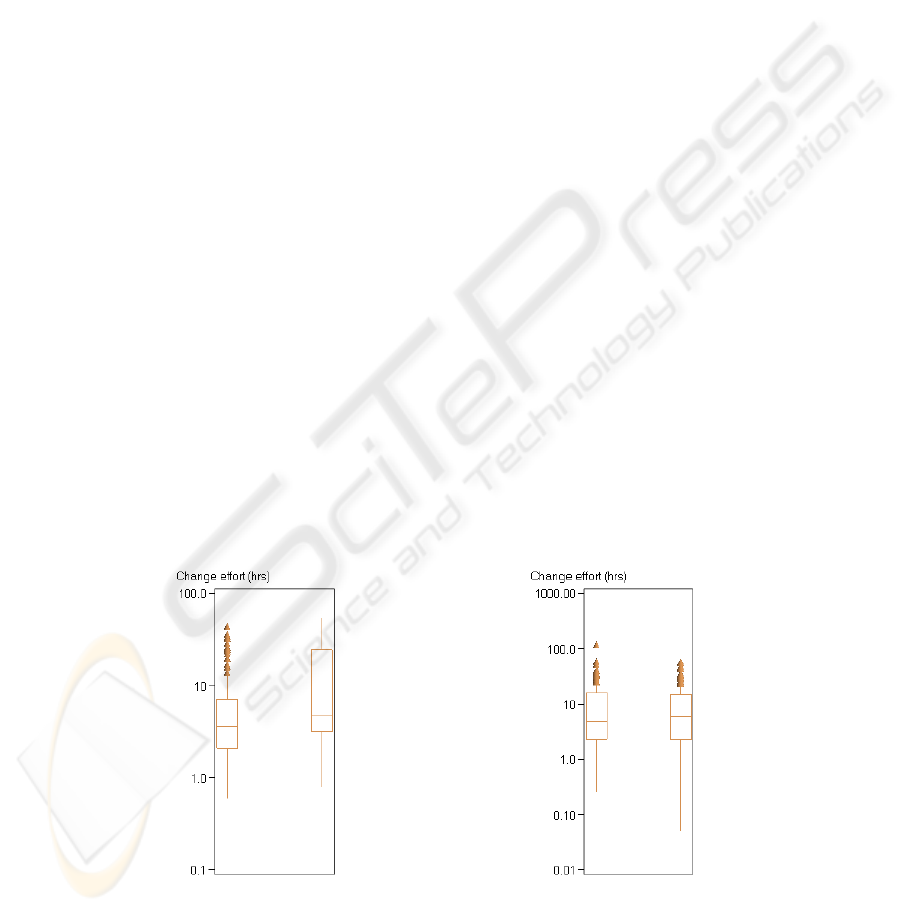
The distribution of change effort in the two periods is shown in Fig. 1 (RCN) and Fig.
2 (MT). The square boxes include the mid 50% of the data points. A log scale is used
on the y-axis, with units in hours. Triangles show outliers in the data set.
For RCN, the plots for the two periods are very similar. The Hodges-Lehmann es-
timate of difference between two data sets (8) is 0, and the associated statistical test
does not indicate a difference between the two periods. For MT, the plots show a
trend towards higher change effort values in
P1. The Hodges-Lehmann estimate is
plus one hour in
P1, and the statistical test showed that the probability is 0.21 that this
result was obtained by pure chance.
Fig. 1. Change effort in RCN, P0 (left) vs. P1. Fig. 2. Change effort in MT, P0 (left) vs. P1.
170

If there were systematic differences in the properties of the change tasks between
the periods, ICPR
1
can be misleading. This was assessed by comparing values for
variables that capture certain important properties. The results are shown in Table 3
and Table 4. The Wilcoxon rank-sum test determined whether changes in these va-
riables were statistically significant. In the case of
isCorrective, the Fischer’s exact
test determined whether the proportion of corrective change tasks was significantly
different in the two periods.
For RCN,
chLoc significantly increased between the periods, while there were no
statistically significant changes in the values of other variables. This indicates that
larger changes were completed in
P1, and that the indicated gain in productivity is a
conservative estimate
For MT,
crTracks significantly decreased between P0 and P1, while addCC and
components increased in the same period. This indicates that more complex changes
were completed in
P1, but that there was less uncertainty about requirements. Be-
cause these effects counteract, it cannot be determined whether the value for ICPR
1
is
conservative. This motivates the use of ICPR
2
and ICPR
3
, which explicitly control for
changes in the mentioned variables.
Table 3. Properties of change tasks in RCN.
Variable P0 P1 p-value
chLoc (mean) 26 104 0.0004
crWords (mean) 107 88 0.89
filetypes (mean) 2.7 2.9 0.50
isCorrective (%) 38 39 0.90
Table 4. Properties of change tasks in MT.
Variable P0 P1 p-value
addCC (mean) 8.7 44 0.06
components (mean) 3.6 7 0.09
crTracks (mean) 4.8 2.5 <0.0001
systExp (mean) 1870 2140 0.43
3.2 Validation of ICPR
2
ICPR
2
is obtained by fitting a model of change effort on change task data from P0
and
P1. The model includes a binary variable representing period of change (inP1) to
allow for a constant proportional difference in change effort between the two periods.
The statistical significance of the difference can be observed directly from the p-value
of that variable. The fitted regression expressions for RCN and MT were:
.1inP10.0veisCorrecti79.0
changed00073.0filetypes2258.0crWords0018.05.9)effortlog(
⋅−⋅
−
⋅
+
⋅
+
⋅+
=
(14)
171

.1inP40.0systExp00013.0
components098.0addCC0041.0crTracks088.01.9)effortlog(
⋅+⋅
−
⋅
+
⋅
+
⋅+
=
(15)
The p-value for
inP1 is low (0.054) for MT and high (0.44) for RCN. All the other
model variables have p-values lower than 0.05. For MT, the interpretation is that
when these model variables are held constant, change effort increases by 50%
(e
0.40
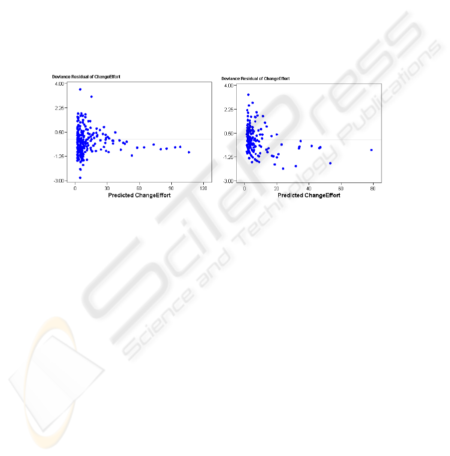
=1.50). A plot of deviance residuals in Fig. 3 and Fig. 4 is used to assess whether
the modelling framework (GLM with gamma distributed change effort and log link
function) was appropriate. If the deviance residuals increase with higher outcomes
(overdispersion) the computed p-values would be misleading. The plots show no sign
of overdispersion. This validation increases the confidence in this indicator for
project MT. For project RCN, the statistical significance is too weak to allow confi-
dence in this indicator alone.
Fig. 3. Residual plot for RCN model (14). Fig 4. Residual plot for MT model (15).
3.3 Validation of ICPR
3
ICPR
3
compares change effort in P1 with the model-based estimates for the same
change tasks had they been completed in
P0. The model was fitted on data from P0.
Fig. 5 shows that actual change effort tends to be higher than estimated effort for MT,
while the tendency is opposite for RCN. For RCN, the low p-value shows that that
actual change effort is systematically lower than the model-based estimates. For
project MT, the high p-value means that actual effort was not systematically higher.
If the variable subset is overfitted to data from P0, the model-based estimates using
data from P1 can be misleading. To evaluate the stability of the model structure, we
compared the model residuals in the
P0 model with those in a new model fitted on
data from
P1 (using the same variable subset). For MT, the model residuals were
systematically larger (Wilcoxon rank-sum test, p=0.0048). There was no such trend
for RCN (Wilcoxon rank-sum test, p=0.78), indicating a more stable model structure.
Another possible problem with ICPR
3
is that model estimates can degenerate for
variable values poorly covered by the original data set. Inspection of the distributions
for the independent variables showed that there was a potential problem with the
variable
chLoc, also indicated by the large difference in mean, shown in Table 3. We
172

re-calculated ICPR
3
after removing the 10 data points that were poorly covered by the
original model, but this did not affect the value of the indicator.
Fig. 5. Model estimates subtracted from actual effort.
In summary, the validation for ICPR
3
gives us high confidence in the result for
project RCN, due to high statistical significance, and evidence of a stable underlying
model structure. For project MT, the opposite conclusion applies.
3.4 Validation of ICPR
4
ICPR
4
is obtained by comparing the estimates that were made in the benchmarking
sessions in
P0 and P1. Fig. 6 shows that for project MT, the estimates tended to be
higher in
P1 than in P0. For project RCN, there was no apparent difference.
A two-sided sign determines whether the differences are positive or negative in
more cases than could be expected by pure chance. For project MT, the low p-value
shows that estimates in
P1 are systematically higher than estimates in P0. For project
RCN, the high p-value means that estimates in
P1 were not systematically different
from in
P0.
A change in estimation accuracy constitutes a threat to the validity of ICPR
4
. For
example, if developers tended to underestimate changes in
P0, experience may have
taught them to provide more relaxed estimates in
P1. Because this would apply to real
change tasks as well, we evaluated this threat by comparing estimation accuracy for
real changes between the periods. The required data for this computation (developers’
estimates and actual change effort) was only available for RCN. Fig. 7 shows a dif-
ference in estimation bias between the periods (Wilcoxon rank-sum test, p=0.086).
Changes tended to be overestimated in
P0 and underestimated in P1. Hence, the
developers became more optimistic, indicating that ICPR
4
can be biased towards a
higher value. This agrees with the results for the other indicators.
In summary, the benchmarking sessions supported the results from data on real
change tasks. An additional result from the benchmarking session was that uncertain-
ty estimates consistently increased between the periods in both projects. The develop-
ers explained this result by claiming they were more realistic in their assessments of
uncertainty.
173

Fig. 6. Differences in estimates.
Fig. 7. RCN: Estimates subtracted from actual
effort.
4 Discussion
The described approach to measuring productivity of software processes has some
notable features compared with earlier work in this area. First, rather than searching
for generally valid indicators of productivity, we believe it is more realistic to devise
such indicators within more limited scopes. Our indicators target situations of soft-
ware evolution where comparable change tasks are performed during two time inter-
vals that are subject to the assessment. Second, rather than attempting to assess gen-
eral validity, we believe it is more prudent to integrate validation procedures with the
indicators. Third, our indicators are flexible within the defined scope, in that the
structure of the underlying change effort models can vary in different contexts.
In a given project context, it may not be obvious which indicator will work best.
Our experience is that additional insight was gained about the projects from using and
assessing several indicators. The three first indicators require that data on change
effort from individual change tasks is available. The advantage of ICPR
1
is that data
on change effort is the
only requirement for data collection. The caveat is that addi-
tional quantitative data is needed to assess the validity of the indicator. If this data is
not available, a development organization may choose to be more pragmatic, and
make qualitative judgments about potential differences in the properties of change
tasks between the periods.
ICPR
2
and ICPR
3
require projects to collect data about factors that affect change
effort, and that statistical models of change effort are established. To do this, it is
essential to track relationships between change requests and code changes committed
to the version control system. An advantage of ICPR
3
is that any type of prediction
framework can be used to establish the initial model. For example, data mining tech-
niques such as decision trees or neural networks might be just as appropriate as mul-
tiple regression. Once the model is established, spreadsheets can be used to generate
the estimates, construct the indicator and perform the associated statistical test.
ICPR
2
relies on a statistical regression model fitted on data from the periods under
consideration. This approach better accounts for underlying changes in the cost driv-
ers between the periods, than does ICPR
3
. In organizations with a homogenous
174

process and a large amount of change data, the methodology developed by Graves
and Mockus could be used to construct the regression model [17]. With their ap-
proach, data on development effort need only be available on a more aggregated level
(e.g., monthly), and relationships between change requests and code commits need
not be explicitly tracked.
ICPR
4
most closely approximates the hypothetical measure of comparing change
effort for identical change tasks. However, it can be difficult to design benchmarking
tasks that resemble real change tasks, and to evaluate whether changes in estimation
accuracy have affected the results. If the benchmarking sessions are organized fre-
quently, developers’ recollection of earlier estimates would constitute a validity
threat.
As part of our analysis, we developed a collection of scripts to retrieve data, con-
struct basic measures and indicators, and produce data and graphics for the evalua-
tion. This means that it is straightforward and inexpensive to continue to use the indi-
cators in the studied projects. It is conceptually straightforward to streamline the
scripts so that they can be used with other data sources and statistical packages.
5 Conclusions
We conducted a field study in two software organizations to measure productivity
changes between two time periods. Our perspective was that productivity during
software evolution is closely related to the effort required to complete change tasks.
Three of the indicators used the same data from real change tasks, but different me-
thods to control for differences in the properties of the change tasks. The fourth indi-
cator compared estimated change effort for a set of benchmarking tasks designed to
be representative of real change tasks.
The indicators suggested that productivity trends had opposite directions in the two
projects. It is interesting that these findings are consistent with major changes and
events in the two projects: Between the measured periods, the project with the indi-
cated higher productivity performed a reorganization of their system with the goal of
simplifying further maintenance and evolution. The project with indicated lower
productivity had changed from fixed-price maintenance contracts to time-and-
material contracts, which may have relaxed the time pressure on developers.
The paper makes a contribution towards the longer term goal of using methods and
automated tools to assess trends in productivity during software evolution. We be-
lieve such methods and tools are important for software projects to assess and optim-
ize development practices.
Acknowledgements
We thank Esito AS and KnowIT Objectnet for providing us with high quality empiri-
cal data, and the Simula School of Research and Innovation for funding the research.
175

References
1. Eick, S.G., Graves, T.L., Karr, A.F., Marron, J.S., and Mockus, A.: Does Code Decay?
Assessing the Evidence from Change Management Data. IEEE Transactions on Software
Engineering, 27(1) (2001) 1-12
2. DeMarco, T. and Lister, T.: Human Capital in Peopleware. Productive Projects and Teams.
Dorset House Publishing, (1999) 202-208
3. Mens, T. and Tourwé, T.: A Survey of Software Refactoring. IEEE Transactions on Soft-
ware Engineering, 30(2) (2004) 126-139
4. Dybå, T., Arisholm, E., Sjøberg, D.I.K., Hannay, J.E., and Shull, F.: Are Two Heads Better
Than One? On the Effectiveness of Pair Programming. IEEE Software, 24(6) (2007) 12-15
5. Tonkay, G.L.: Productivity in Encyclopedia of Science & Technology. McGraw-Hill,
(2008)
6. Fenton, N.E. and Pfleeger, S.L.: Measuring Productivity in Software Metrics, a Rigorous &
Practical Approach. (1997) 412-425
7. Ramil, J.F. and Lehman, M.M.: Cost Estimation and Evolvability Monitoring for Software
Evolution Processes. Proceedings of the Workshop on Empirical Studies of Software Main-
tenance (2000)
8. Abran, A. and Maya, M.: A Sizing Measure for Adaptive Maintenance Work Products.
Proceedings of the International Conference on Software Maintenance (1995) 286-294
9. Albrecht, A.J. and Gaffney Jr, J.E.: Software Function, Source Lines of Code, and Devel-
opment Effort Prediction: A Software Science Validation. IEEE Transactions on Software
Engineering, 9(6) (1983) 639-648
10. Maya, M., Abran, A., and Bourque, P.: Measuring the Size of Small Functional Enhance-
ments to Software. Proceedings of the 6th International Workshop on Software Metrics
(1996)
11. DeMarco, T.: An Algorithm for Sizing Software Products. ACM SIGMETRICS Perfor-
mance Evaluation Review, 12(2) (1984) 13-22
12. Ramil, J.F. and Lehman, M.M.: Defining and Applying Metrics in the Context of Continu-
ing Software Evolution. Proceedings of the Software Metrics Symposium (2001) 199-209
13. Abran, A. and Hguyenkim, H.: Measurement of the Maintenance Process from a Demand-
Based Perspective. Journal of Software Maintenance: Research and Practice, 5(2) (1993)
63-90
14. Rombach, H.D., Ulery, B.T., and Valett, J.D.: Toward Full Life Cycle Control: Adding
Maintenance Measurement to the SEL. Journal of Systems and Software, 18(2) (1992) 125-
138
15. Stark, G.E.: Measurements for Managing Software Maintenance. Proceedings of the 1996
International Conference on Software Maintenance (1996) 152-161
16. Arisholm, E. and Sjøberg, D.I.K.: Towards a Framework for Empirical Assessment of
Changeability Decay. Journal of Systems and Software, 53(1) (2000) 3-14
17. Graves, T.L. and Mockus, A.: Inferring Change Effort from Configuration Management
Databases. Proceedings of the 5th International Symposium on Software Metrics (1998)
267–273
18. Kitchenham, B. and Mendes, E.: Software Productivity Measurement Using Multiple Size
Measures. IEEE Transactions on Software Engineering, 30(12) (2004) 1023-1035
19. Schwaber, K.: Scrum Development Process. Proceedings of the 10th Annual ACM Confe-
rence on Object Oriented Programming Systems, Languages, and Applications (1995) 117-134
20. Benestad, H.C., Anda, B., and Arisholm, E.: An Investigation of Change Effort in Two
Evolving Software Systems. Technical report 01/2009 (2009) Simula Research Laboratory
21. Grimstad, S. and Jørgensen, M.: Inconsistency of Expert Judgment-Based Estimates of
Software Development Effort. Journal of Systems and Software, 80(11) (2007) 1770-1777
176