Clustering and Density Estimation for Streaming Data
using Volume Prototypes
Maiko Sato, Mineichi Kudo and Jun Toyama
Division of Computer Science
Graduate School of Information Science and Technology, Hokkaido University
Kita-14, Nishi-9, Kita-ku, Sapporo 060-0814, Japan
Abstract. The authors have proposed volume prototypes as a compact expression
of a huge data or a data stream, along with a one-pass algorithm to find them. A
reasonable number of volume prototypes can be used, instead of an enormous
number of data, for many applications including classification, clustering and
density estimation. In this paper, two algorithms using volume prototypes, called
VKM and VEM, are introduced for clustering and density estimation. Compared
with the other algorithms for such a huge data, we showed that our algorithms
were advantageous in speed of processing, while keeping the same degree of per-
formance, and that both applications were available from the same set of volume
prototypes.
1 Introduction
In these years, we often deal with an enormous amount of data or a data stream in a large
variety of pattern recognition tasks. Such data require a huge amount of memory space
and computation time for processing. So it is preferable to find a compact expression
of data that is acceptable in time and space without losing characteristics of original
datasets. For this goal, we have proposed volume prototypes [1, 2] as an extension of
conventional point prototypes. Each of volume prototypes is a geometric configuration
that represents many data points inside.
Volume prototypes can be generated by a single-pass algorithm, and thus they are
significantly effective for streaming data that can be accessed only once. As another ad-
vantage, volume prototypes typically converge to modes of the underlying distribution,
so that we do not need to determine the number of prototypes beforehand. It suffices to
take a sufficiently large number of initial prototypes, unlike mixture models.
In our earlier studies [1, 2], we conducted some experiments and analyzed a typical
behavior of volume prototypes. In this paper, we investigate the applicability of volume
prototypes. Especially, we try to apply volume prototypes to clustering and construction
of mixture models.
2 Related Works
There have been many studies of clustering and density estimation for huge datasets or
data streams.
Sato M., Kudo M. and Toyama J. (2009).
Clustering and Density Estimation for Streaming Data using Volume Prototypes.
In Proceedings of the 9th International Workshop on Pattern Recognition in Information Systems, pages 39-48
DOI: 10.5220/0002173500390048
Copyright
c
 SciTePress

Density estimation algorithms for a huge dataset are found in the literature [3–6].
Zhang et al. extended a kernel method to achieve a fast density estimation for very
large databases [3]. Arandjelovi´c and Cipolla realized a real-time density estimation by
incremental learning of GMM [4]. The incremental EM algorithm [5] attempts to reduce
the computational cost needed by EM algorithm. This is made by adopting partial E-
steps. It divides a whole dataset into some blocks and performs a partial E-step on
each block in a cyclic way. The lazy EM algorithm [6] has the same strategy with the
incremental EM algorithm. However, it performs a partial E-step only on a significant
subset of data.
Clustering methods for a huge dataset are also seen in the literature [7–10]. Charikar
et al. proposed a one-pass clustering algorithm in a streaming model [7]. It produces
a constant factor approximation of the solution of the k-median problem in storage
space O(k poly log n) for size n data. Bradley et al. showed an efficient clustering
method for large databases [8]. Their method is based on classifying regions into three
kinds of regions: the regions that must be maintained as they are, the regions that are
compressive, and the regions that can be discarded. This algorithm requires at most one
scan of the database. The algorithm BIRCH [9] by Zhang et al. achieves an efficient
clustering for a huge dataset by constructing a CF-tree that is a hierarchical summary of
clusters. Data is scanned only once to construct a CF-tree. The algorithm FEKM [10]
by Goswami et al. produces almost the same clusters as the original k-means algorithm.
Their algorithm is basically one-pass, and obtain clusters close to the correct clusters of
the k-means with a few number of additional scans.
These approaches would be effective for a huge dataset in several situations. How-
ever, some of them require to keep a whole data and others require a constant number
of rescanning of data or its reduced subset. If we are allowed to access each data only
once, some of these methods are not available. One more important thing is that we do
clustering for one goal, e.g., data compression, do density estimation for another goal,
e.g., classification, and sometimes we do both. In this case, it is desirable to be able
to carry out both efficiently. The goal of this paper is to show that our approach using
volume prototypes gives one of possible solutions.
3 Algorithm for Volume Prototypes
In this section, we show the concrete algorithm VP to generate volume prototypes. The
single-pass algorithm is shown in Fig. 1.
The outline is as follows. With multiple scans over the first N samples in different
M orders, we obtain M seed prototypes (ME Step). Here N is relatively small, say
N = 500, and M is taken to be ten times or so the number of expected modes, say
M = 100. We bring up those seed prototypes by updating them using the samples
fell in their acceptance regions (C Step). For final prototypes, we carry out prototype
selection using greedy set covering to have L final prototypes.
3.1 Details
Dataset: We consider a data stream x
1
, x
2
, . . . , x
N
, x
N+1
, . . . of d-dimensional vec-
tors.
40

Inputs:(Unlimited samples) x
1
, x
2
, . . . , x
N
, . . .
N is the number of samples for ME Step.
M is the number of seed prototypes.
N
v
is the number of latest samples to be kept.
θ is the value to determine radius r of the acceptance region.
Procedure for obtaining volume prototypes
ME (mode estimation) step:
Repeat M times the following for the first N samples.
1. Choose a random permutation σ to reorder the samples to x
σ
1
, x
σ
2
, . . . , x
σ
N
.
2. Initialize a prototype by the way described in the detailed description.
3. Use x
σ
2
, . . . , x
σ
N
in order to update the seed prototype by the same way as 2.
(using only the samples in the acceptance region (1)).
C (Convergence) step:
For each sample x
i
(i = N + 1, N + 2, . . .) do the following.
1. Update the seed prototypes in which x
i
falls by (2)–(4).
2. Keep the latest N
v
samples.
Exploit time:
From M prototypes, select greedily L(≤ M) prototypes until no improvement is
found for covering N
v
samples. Count the number of samples falling in each pro-
totype in N
v
samples. Here a sample is divided by k when k prototypes share it.
Fig. 1. Volume Prototype Algorithm (VP).
Prototype: Let p = (µ, Σ, r, n) be a prototype. Here, µ is the prototype center, Σ is
the covariance matrix, r is the Mahalanobis radius and n is the number of samples
inside the prototype.
Included Sample Set: Let S
p
be the set of data points inside prototype p, which is
specified by S
p
= {x
i
|(x
i
− µ)
0
Σ
−1
(x
i
− µ) ≤ r
2
}. Then n = |S
p
|. We
approximate n by the number of samples used for updating the prototype.
Acceptance Region: We specify the acceptance region A
p
of prototype p = (µ, Σ, r, n)
by the acceptance Mahalanobis radius R as
A
p
= {x|(x − µ)
0
Σ
−1
(x − µ) ≤ R
2
}. (1)
Here, R(≥ r) is determined from r and n by R = r +
q
χ
2
d
(0.95)
n
.
Updating Procedure: When a sample x falls into the acceptance region A
(t)
p
of pro-
totype p
(t)
at (t + 1)th update, p
(t)
is updated to p
(t+1)
by
n
(t+1)
= n
(t)
+ 1, (2)
µ
(t+1)
=
1
n
(t+1)

n
(t)
µ
(t)
+ x

, (3)
Σ
(t+1)
=
1
n
(t+1)

n
(t)
Σ
(t)
+ xx
0
+ n
(t)
µ
(t)
µ
(t)0
− n
(t+1)
µ
(t+1)
µ
(t+1)0

.(4)
The radius R of the acceptance region is also updated.
41

Initialization of ME Step: We initialize the center µ
(0)
and the covariance matrix
Σ
(0)
by µ
(0)
= x
1
(the first element after random reordering) and Σ
(0)
= λ
2
I.
Here, λ
2
=
1
dN
P
N
i=1
min
j6=i,j∈{1,2,...,N }
kx
i
− x
j
k
2
(k · k
2
is the squared Eu-
clidean norm) and I is the unit matrix. In addition, we set the initial value of n
(0)
to n
(0)
= d + 1.
4 Applications of Volume Prototypes
Volume prototypes are an intermediate representation between data and clusters, while
they are more akin to data themselves. We can use them for costly applications instead
of a large amount of original samples. In this section, we show two applications for
clustering and density estimation.
Let us assume that we have a huge amount of data and they are represented by a
reasonable number of volume prototypes. In the following, we consider the correspon-
dence between a sample and a volume prototype. A big difference is that the latter has
many samples in it and has a volume specified by a covariance matrix and a Maha-
lanobis radius.
4.1 EM Algorithm with Volume Prototypes (VEM)
We consider first modeling of a given density by a finite mixture of Gaussian com-
ponent densities. The number K of component densities is assumed to be given be-
forehand. Let the kth component be a Gaussian N(x; ν
k
, Σ
k
), where ν
k
is the mean,
Σ
k
is the covariance matrix. Then, the density is estimated by a mixture as f(x) =
P
K
k=1
π
k
N(x; ν
k
, Σ
k
) with prior probabilities π
k
. To estimate the parameter values
from given volume prototypes, we show a volume prototype version (VEM) of EM
algorithm. The concrete algorithm is shown in Fig. 2.
In the following, we use suffix j for volume prototypes and k for component densi-
ties. Thus, jth volume prototype is denoted by p
j
= (µ
j
, Σ
j
, n
j
), omitting the radius
r
j
.
In the Maximization step (M step), we estimate the mean and covariance of kth
component density from the currently estimated membership value m
k
(p) of a volume
prototype p to kth component. Here,
P
K
k=1
m
k
(p) = 1. The parameter values are
estimated by the maximum likelihood estimators. The updating procedure is given as
π
k
=
X
j
m
k
(p
j
)n
j
/
X
j
n
j
, ν
k
=
X
j
m
k
(p
j
)n
j
µ
j
/
X
j
m
k
(p
j
)n
j
Σ
k
=
X
j
m
k
(p
j
)n
j
{Σ
j
+ (µ
j
− ν
k
) (µ
j
− ν
k
)
0

/
X
j
m
k
(p
j
)n
j
.
In the Expectation step (E step), we re-estimate the membership values m
k
(p) from
the currently estimated K component densities. To do this, we use a kind of distance
measure between p and kth component. In the original EM algorithm, Mahalanobis
42

Inputs: L volume prototypes: p
1
, p
2
, . . . , p
L
(p
l
= (µ
l
, Σ
l
, n
l
), l = 1, 2, . . . , L).
K is the number of components.
Outputs: f(x) =
P
K
k=1
π
k
f
k
(x; θ
k
) (f
k
is a Gaussian with θ
k
= (ν
k
, Σ
k
) ).
Procedure for obtaining a mixture model
Initialize step:
Set randomly the membership m
k
(p
l
) for every kth component and lth prototype.
Repeat the following M step and E step in turn until convergence.
M step: For kth component (k = 1, 2, . . . , K), update the following:
π
k
=
P
l
m
k
(p
l
)n
l
/
P
l
n
l
ν
k
=
P
l
m
k
(p
l
)n
l
µ
l
/
P
l
m
k
(p
l
)n
l
Σ
k
=
P
l
m
k
(p
l
)n
l
{Σ
l
+ (µ
l
− ν
k
) (µ
l
− ν
k
)
0
} /
P
l
m
k
(p
l
)n
l
.
E step: For lth prototype (l = 1, 2, . . . , L), update the membership by
m
k
(p
l
) = π
k
(2π)
−
D
2
|Σ
k
|
−
1
2
e
−
1
2
(
trΣ
−1
k
Σ
l
+(µ
l
−ν
k
)
0
Σ
−1
k
(µ
l
−ν
k
)
)
.
Fig. 2. Volume prototype EM algorithm (VEM).
Inputs: L volume prototypes: p
1
, p
2
, . . . , p
L
; K is the number of clusters to be found.
Outputs: K clusters specified by means ν
1
, ν
2
, . . . , ν
K
.
Procedure K-means with volume prototypes
t ← 0.
Choose the first K prototypes and assign their centers to ν
(0)
1
, ν
(0)
2
, . . . , ν
(0)
K
.
Repeat the following until convergence.
Assign prototype p
l
(l = 1, 2, . . . , L) to the nearest cluster C
s
with ν
(t)
s
.
Here, the nearness between p
l
= (µ
l
, Σ
l
, n
l
) and ν
(t)
s
is measured by ||ν
(t)
s
− µ
l
||.
t ← t + 1.
Update ν
(t)
k
(k = 1, 2, . . . , K) by ν
(t)
k
=
1
N
k
P
p
l
∈C
k
n
l
µ
l
, where N
k
=
P
p
l
∈C
k
n
l
.
Fig. 3. Volume prototype k-means algorithm (VKM).
distance between a sample x and mean ν
k
is used. Here, since p has a volume, we use
the expected Mahalanobis distance on prototype p:
E
X∈p
j
(X − ν
k
)
0
Σ
−1
k
(X − ν
k
)
= E
X∈p
j
(X − µ
j
+ µ
j
− ν
k
)
0
Σ
−1
k
(X − µ
j
+ µ
j
− ν
k
)
= trΣ
−1
k
Σ
j
+ (µ
j
− ν
k
)
0
Σ
−1
k
(µ
j
− ν
k
).
Then, with the prior probability π
k
, the membership value is updated as
m
k
(p
j
) = π
k
(2π)
−
D
2
|Σ
k
|
−
1
2
· exp

−
1
2

trΣ
−1
k
Σ
j
+ (µ
j
− ν
k
)
0
Σ
−1
k
(µ
j
− ν
k
)


.
Here, we notice that the estimated Mahalanobis distance converges to the ordinal Ma-
halanobis distance (µ
j
− ν
k
)
0
Σ
−1
k
(µ
j
− ν
k
) of a single point µ
j
under the assumption
that Σ
j
= I and  → 0. Therefore, this way of assigning membership values is an
extension of the traditional E step.
43

4.2 k-means Algorithm with Volume Prototypes (VKM)
It is also easy to make the k-means algorithm applicable to volume prototypes (VKM).
Here, it is also assumed that the number K of clusters is determined beforehand.
When J volume prototypes {p
j
= (µ
j
, Σ
j
, n
j
)} (j = 1, 2, . . . , J) are combined
into one, we have a combined volume prototype p = (µ, Σ, n):
n =
J
X
j=1
n
j
, µ =
J
X
j=1
n
j
n
µ
j
Σ =
J
X
j=1
n
j
n

Σ
j
+ (µ
j
− µ)(µ
j
− µ)
0

(5)
These hold even if {p
j
} are samples {x
j
} (easily verified with Σ
j
= 0, µ
j
= x
j
and
n
j
= 1).
For extending k-means using samples to the one using volume prototypes, all we
need is to define the distance between a volume prototype and a cluster center. Under
the assumption that a volume prototype (and all samples in it) belongs to one cluster
only, the squared distance minimization criterion Q for samples in the original k-means
can be used even for volume prototypes:
Q =
K
X
k=1
X
x∈C
k
||x − ν
k
||
2
=
K
X
k=1
X
x∈C
k
tr(x − ν
k
)(x − ν
k
)
0
(C
k
is kth cluster)
=
K
X
k=1
X
p
j
∈C
k
n
j

trΣ
j
+ ||µ
j
− ν
k
||
2

(Eq. (5))
=
X
p
j
n
j
trΣ
j
+
K
X
k=1
X
p
j
∈C
k
n
j
||µ
j
− ν
k
||
2
.
The first term is the irreducible error when volume prototypes are used. Therefore,
when we adopt the k-means algorithm to find a sub-optimal solution of this optimiza-
tion problem, we may assign a volume prototype to the nearest cluster in the dis-
tance ||µ
j
− ν
k
||. By setting
∂Q
∂ν
k
= 0, we have the estimated mean for iteration:
ν
k
=
1
N
k
P
p
j
∈C
k
n
j
µ
j
, where N
k
=
P
p
j
∈C
k
n
j
. The concrete algorithm is shown
in Fig. 3.
In algorithm VKM, the cluster centers can be initialized by the first K prototypes.
This strategy is effective because these K prototypes are already chosen in VP algo-
rithm so as to cover as many samples as possible in order.
5 Experiments
In the following experiments, we used three 2-dimensional artificial datasets:
1. Circle: Two clusters. One cluster is concentrated on the origin and it is surrounded
by the other cluster at a distance.
44

2. 4-Cross: Four Gaussians that cross at four corners.
3. 5-Gaussian: Five Gaussians. Some of them are close.
In each dataset, 100,000 samples were generated according to a specified distribution.
We chose M = 100 seed volume prototypes with radius r = χ
2
2
(0.9) in VP algorithm.
The first N = 1000 samples were used for ME step and prototype selection.
The obtained volume prototypes are shown in Fig.4 (1st column). In Fig.4, only
selected volume prototypes are shown. Therefore, the number L is rather less than M =
100. We can see that 1) the set of volume prototypes represents well the distribution, 2)
they are located inside the distribution because of θ = 0.9, and 3) the number (25, 23
and 24 in order) is quite smaller than the number 10
5
of samples.
5.1 Experiment 1 : Clustering
We applied our VKM clustering method to the selected final prototypes. We compared
it with a one-pass k-means algorithm, SKM (scalable k-means) [11]. SKM was applied
to all the data. We examined two different numbers of clusters. The results are shown
in Fig.4 (2nd and 3rd columns).
From Fig.4, we see:
1. When the specified number K of clusters is the same as that of the underlying
distribution, the cluster centers are comparable between VKM and SKM.
2. If K is larger than the correct number, the cluster centers found by VKM are located
inside the distribution compared with those by SKM.
5.2 Experiment 2 : Mixture Models
Then, we applied our VEM method to the same selected final prototypes. We used
the results of VKM for initializing the membership values of a mixture model. We
compared it with the incremental EM algorithm [5]. In the incremental EM algorithm,
the number of blocks over which a partial E-step was carried was set to 100. Two
different numbers of components were examined. The results are also shown in Fig.4
(4th and 5th columns).
From Fig.4, we see the following:
1. The incremental EM and VEM are almost comparable when K is correct.
2. If K is larger, the components found by VEM are more safely secured than those of
the incremental EM. Note that the number of components is automatically reduced
to a near optimal number. This is because volume prototypes limit an excessive
production of small, in the number of included samples, components (see the results
of 4-Cross with K = 8 and 5-Gaussian with K = 10).
3. The components obtained by VEM are narrower than those of the incremental EM.
This is because the components in VEM are generated from volume prototypes that
give an inner approximation of the distribution.
In total, our VEM algorithm is more stable compared with the incremental EM
algorithm.
45

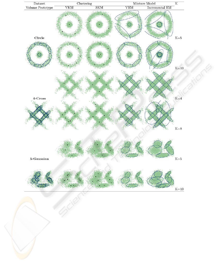
Fig. 4. Results of clustering and mixture models in three datasets (θ = 0.90). In clustering,
the cluster centers are shown as black dots. In mixture models, the covariance matrix of each
component is shown.
5.3 Computation Time
The calculation time is shown in Table 1. It is clear that our two algorithms of VKM and
VEM are faster than SKM and the incremental EM algorithm, respectively, as long as
we do not take into account the time consumed for obtaining volume prototypes. Even
if we add the time for obtaining volume prototypes, VEM is faster than the incremental
EM. The time advantage of VKM and VEM would be increased if we use a larger
46

Table 1. Time comparison in clustering and mixture models.
Dataset K Time (sec.)
VP VKM SKM VEM Incremental EM
Circle 5 5.908 0.001 4.204 0.012 10.136
(25 prototypes) 10 — 0.004 4.216 0.048 19.133
4-Cross 4 7.440 0.001 2.204 0.028 7.732
(23 prototypes) 8 — 0.001 2.532 0.184 15.332
5-Gaussian 5 7.928 0.001 2.544 0.012 9.808
(24 prototypes) 10 — 0.008 3.520 0.104 18.825
dataset, because VP is a completely one-pass algorithm. It should be noted that VKM
and VEM are separately applicable to the same set of volume prototypes. In addition,
we can try several values of K very efficiently with VKM and VEM for model selection.
6 Conclusions
In this paper, we have presented two algorithms for clustering and density estimation on
the basis of volume prototypes which can be used instead of a huge data and obtained
by a single-pass algorithm. The necessary number of volume prototypes is quite smaller
than the number of given samples, therefore, our algorithms work very efficiently for a
huge data or data streams.
One of proposed algorithms is a volume prototype version (VEM) of EM algorithm.
It is for density estimation. Since each prototype has a volume, we extended the original
algorithm so as to take into account the volume and the number of samples included.
Another algorithm is a k-means algorithm for volume prototypes (VKM). In this al-
gorithm, we developed a distance measure between a volume prototype and a cluster
center as a natural extension of its point version.
We confirmed the efficiency of both algorithms in some experiments with 2 - di-
mensional artificial data. The main advantage of these algorithms is that we can carry
out both algorithms in low cost, once volume prototypes are given. We will further
investigate the applicability for high-dimensional real-world datasets.
References
1. Tabata, K., Kudo, M.: Information compression by volume prototypes. The IEICE Technical
Report, PRMU, 106 (2006) 25–30 (in Japanese)
2. Sato, M., Kudo, M., Toyama, J.: Behavior Analysis of Volume Prototypes in High Dimen-
sionality. In: Structural, Syntactic and Statistical Pattern Recognition, Lecture Notes in Com-
puter Science. Volume 5342., Springer (2008) 884–894
3. Zhang, T., Ramakrishnan, R., Livny, M.: Fast density estimation using CF-kernel for very
large databases. Proceedings of the fifth ACM SIGKDD international conference on Knowl-
edge discovery and data mining (1999) 312–316
4. Arandjelovic
´
c, O., Cipolla, R.: Incremental learning of temporally-coherent Gaussian mix-
ture models. Proceedings of the IAPR British Machine Vision Conference (2005) 759–768
5. Neal, R.M., Hinton, G.E.: A view of the EM algorithm that justifies incremental, sparse, and
other variants. Learning in Graphical Models (1999) 355–368
47

6. Thiesson, B., Meek, C., Heckerman, D.: Accelerating EM for Large Databases. Machine
Learning 45 (2001) 279–299
7. Charikar, M., O’Callaghan, L., Panigrahy, S.U.R.: Better Streaming Algorithms for Cluster-
ing Problems. Proceedings of the thirty-fifth annual ACM symposium on Theory of comput-
ing (2003) 30–39
8. Bradley, P.S., Fayyad, U.M., Reina, C.A.: Scaling clustering algorithms to large databases.
Knowledge Discovery and Data Mining (1998) 9–15
9. Zhang, T., Ramakrishnan, R., Livny, M.: Birch: an efficient data clustering method for very
large databases. SIGMOD Rec., 25 (1996) 103–114
10. Goswami, A., Jin, R., Agrawal, G.: Fast and exact out-of-core k-means clustering. IEEE
International Conference on Data Mining (2004) 83–90
11. Farnstrom, F., Lewis, J., Elkan, C.: Scalability for clustering algorithms revisited. SIGKDD
Explor. Newsl., 2 (2000) 51–57
48