
Topologies and Meaning Generating Capacities of
Neural Networks
Jürgen Klüver and Christina Klüver
Department of Economy - COBASC Research Group, University of Duisburg-Essen
Universitätsstr. 12, 45117 Essen, Germany
Abstract. The paper introduces the concept of meaning generating capacity
(MC) of neural nets, i.e. a measure of information processing, depending on the
size of basins of attraction. It can be shown that there is a significant relation
between the variance values of the weight matrix of a network and its MC-
values. By the concept of MC network characteristics like robustness and
generalizing capability can be explained.
1 Introduction
The analysis of topological characteristics of complex dynamical systems frequently
enables important insights into the behavior, i.e. the dynamics of such systems. By
“topology” we here mean that set of system’s rules that determine, which elements of
the respective systems interact with which other elements. In the classical
mathematical meaning of topology these rules define the neighborhood relations of
the respective elements, which are at the core of, e.g., the fundamental Hausdorff
axioms of topology. In the case of neural networks the topology is usually defined by
the according weight matrix, which determines the degree of interaction between the
different elements, including the limiting case of interaction degree equal to zero.
In [1] we introduced the concept of the meaning processing capacity (MC) of a
complex dynamical system. This definition was motivated by some informal remarks
of Wolfram [3] about the “information processing capacity” of complex dynamical
systems. With this term Wolfram described the fact that frequently different initial
states of a system generate the same final attractor state; other systems in contrast
generate different final states if the initial states are different. In other words, the
information processing capacity refers to the different sizes of the “basins of
attraction” of a system, i.e. the sets of initial states that generate the same final
attractor state.
In [1] we defined the concept of the “meaning” of a message by the final attractor
state a system generates when receiving this message; in other words, a system
processes a message and generates an according meaning. Therefore, we now use the
term of meaning generating capacity (MC), i.e. the capacity to generate more or less
different meanings when receiving different inputs.
The MC-value of a complex dynamical system is now defined as the proportion
between the size m of the set of all final attractor states and the size n of the set of all
Klüver J. and Klüver C. (2009).
Topologies and Meaning Generating Capacities of Neural Networks.
In Proceedings of the 5th International Workshop on Artificial Neural Networks and Intelligent Information Processing, pages 13-22
DOI: 10.5220/0002261600130022
Copyright
c
SciTePress

initial states of a system, i.e., MC = m/n. Obviously 0 < MC ≤ 1: MC = 0 is
impossible because each complex system has at least one final state, even if it is an
attractor state with a very large period. The according limiting case hence is MC =
1/n. If MC is very small then many different initial states will generate the same final
states – the according attractors are characterized by large basins of attraction. If MC
= 1 then each different initial state will generate a different final attractor state. This is
the other limiting case, where the basins of attraction all are of size 1. In other words,
small values of MC mean large basins of attractions and vice versa. It must be noted
that we refer only to discrete systems, i.e. systems with only a finite number of initial
states.
There are at least three main reasons why this concept is important: On the one
hand it is possible via the usage of MC to analyze complex dynamical systems like
neural networks with respect to their informational complexity. In this sense MC
allows for new approaches in the theory of computability. On the other hand an
important and frequently mentioned characteristic of neural networks can be
understood in a new and more differentiated way: In all textbooks on neural networks
there are statements like “one of the main advantages of neural networks is their
robustness, i.e. their tolerance with respect to faulty inputs” or something equivalent.
We shall show that via the definition of MC not only a theoretical explanation of this
advantage can be given but also a measurement of this robustness; in particular by the
variation of MC specific neural networks can be generated that are either very robust,
less robust or not at all robust in the sense of error tolerance.
Last but not least it is possible to give by the usage of MC an explanation for
phenomena known from the field of human information processing. It is well known
that different humans react in a significant different way to the same messages. This
can be illustrated by the examples of fanatics who refer all messages to the same
cause, e.g. the enmity of Western Capitalism to religious movements. The psychiatrist
Sacks [2] for another example describes a rather intelligent and well-educated man
who is unable to distinguish little children from fire hydrants. The definition of MC
can be a useful approach to construct mathematical models for the explanation of such
phenomena.
In contrast to dynamical systems like, e.g., cellular automata and Boolean
networks neural networks are not often analyzed in terms of complex dynamical
systems. Therefore, it is necessary to clarify what we understand by “initial states”
and “final attractor states” when speaking of neural networks.
In a strict systems theoretical sense all initial states of neural networks are the
same, i.e. the activation values of all neurons are equal to zero, and regardless to
which layer(s) they belong. Because this fact would make the definition of different
initial states quite useless we define the initial state of a neural net as the state where
the neurons of the input layer have been externally activated with certain input values
and where the activation values of all other neurons still are equal to zero, in
particular those of the output layer. An initial state S
i
of a neural net, hence, is
formally defined by S
i
= ((A
i
), (0)), if (A
i
) is the input vector and (0) is the output
vector, i.e. it denotes the fact that the values of the output neurons are still equal to
zero. If there is no specific input layer then the definition must be understood that
some neurons are externally activated and the others are not.
14

The external activation of the input neurons causes via the different functions the
“spread of information”, determined by the respective weight values. In the case of
simple feed forward networks the final activation values of an output layer are
immediately generated; in the case of feed back networks or recurrent ones the output
is generated in a more complex manner; yet in the end in all cases a certain output
vector is generated, i.e., each neuron of the output layer, if there is any, has obtained a
certain activation value. If there is no distinction between different layers as for
example it is the case with a Hopfield network or an interactive network the output
vector will consist of the final activation values of all neurons. Note that except in the
case of feed forward networks the output vector may be an attractor with a period p >
1. The network will then oscillate between different vectors, i.e. between different
states of the attractor. For theoretical and practical purposes neural networks are
mainly analyzed with respect to the input-output relation. Therefore, we define the
final state
S
f
of a neural network as S
f
= ((A
i
), (A
f
)), if (A
i
) is again the input vector
and (A
f
) the final output vector. If (A
f
) is an attractor with period p > 1, then the
components of (A
f
) consists of ordered sets, i.e. the set of all different activation
values the output neurons obtain in the attractor.
Because in the experiments described below we investigate only the behavior of
feed forward networks with respect to different MC-values, for practical purposes we
just define the final state as the values of the output vector after the external activation
via the input vector. Hence we speak of a large basin of attraction if many different
input vectors generate the same output vector and vice versa. The limiting case MC =
1 for example defines a network where each different input vector generates a
different output vector. Accordingly the case M = 1/n defines a network where
practically all n different input vectors generate the same output vector.
With these definitions it is easy to explain and measure in a formal manner the
characteristics of neural networks with respect to robustness. A robust network, i.e. a
network that is tolerant of faulty inputs, has necessarily a MC-value significantly
smaller than 1. Robustness means that different inputs, i.e. inputs that differ from the
correct one, still will generate the “correct” output, i.e. that output that is generated by
the correct input. That is possible only if some faulty inputs belong to the same basin
of attraction as the correct input; these and only these inputs from this basin of
attraction will generate the correct output. All other faulty inputs transcend the limits
of tolerance with respect to the correct output and will accordingly generate another
output. If MC = 1 or near 1 then the network will not be robust at all for the respective
reasons.
The same explanation can be given for the also frequently quoted capability of
neural networks to “generalize”: In a formal sense the generalizing capability is just
the same as robustness, only looked upon from another perspective. A new input can
be perceived as “similar” or as “nearly the same” as an input that the net has already
learned if and only if the similar input belongs to the same basin of attraction as the
input the network has been trained to remember. In other words, the training process
with respect to a certain vector automatically is also a training process with respect to
the elements of the according basin of attraction. The capability of generalization,
hence, can be understood as the result of the construction of a certain basin of
attraction. Accordingly the generalization capability is again dependent on the MC-
values: if these are small, i.e. if the basins of attraction are rather large, then the
15

network has a comparatively great generalizing capability and vice versa. Because
one network can have only one MC-value it is obvious that systems like the human
brain must have for one and the same perceiving task at least two different networks,
namely one with a great generalization capability, i.e., a small MC-value, and one
with a large MC-value to perceive different inputs as different.
Robustness and generalizing capability of a network, hence, can be “globally”
defined by the according MC-value. Yet there is a caveat: it is always possible to
generate networks via according training methods that are characterized by different
basins of attractions with different sizes. Therefore, the MC-value is not necessarily a
unique measure for the size of all basins of attraction of a particular network. The
term “basin of attraction” refers always only to a certain “equivalence class” of input
vectors, namely a set of input vectors that are equivalent in the sense that they
generate the same attractor. The size of these sets may be quite different for specific
attractors. Hence, the MC-value gives just an average measure with respect to the
different basins of attraction. With respect to some attractors and their generating
inputs the networks may be robust and with respect to others not. Considering that
possibility the concept of MC could also be defined as the difference in size of all
basins of attraction of the networks. Fortunately the results of our present experiments
hint at the fact that in most cases the basins of attraction of a certain networks differ
not much in size. The caveat is necessary for theoretical and methodical reasons but
seems not to be very important in practical contexts.
Concepts like “size of basins of attraction” and “values of meaning generation
capacity” obviously are very useful for the explanation of important characteristics
like robustness or generalizing capability. Yet in a strict sense they are too general
concepts because they only explain the behavior of certain neural networks from very
general characteristics of complex dynamical systems. They do not explain, which
structural characteristics of neural networks may be the reason for specific MC-
values. Hence, these concepts remain, so to speak, on a phenomenological level.
In the beginning of our article we mentioned the fact that frequently certain
topological characte-ristics of complex dynamical explain the behavior of such
systems. The topology of a neural network is mainly expressed in the weight matrix.
Hence the thought suggests itself to look for features of the weight matrix that could
explain the size of basins of attraction and MC-values. In anticipation of our results
we may say that we were successful in the sense that we found some general trends
although no deterministic relations.
2 Two Experimental Series
In the first experimental analysis we used a standard three-layered feed forward
network; we chose this type because it is very frequently used for tasks of pattern
recognition and related problems. Because, as is well known, two layers are not
enough to solve problems of non-linear separableness we took three layers in order to
get results for networks with sufficient efficiency. The input layer consists of 10 units,
the hidden layer of 5 and the output layer of 10 units. Input and output neurons are
binary coded, which results in 2
10
= 1024 possible input patterns. To keep the
experiments as clearly as possible we defined “equivalence classes” of input patterns:
16
all input patterns with the same number of zeroes are members of the same class. By
choosing at random one pattern from each class we obtained 11 different input
patterns. The activation function respectively is the sigmoid function; because of the
three layers we chose as learning rule the standard Back Propagation rule.
The training design was the following: In each step the network was trained to
associate different input patterns with one target pattern; the target pattern was again
chosen at random from the 11 input patterns. In the first step the tasks was to
associate each input pattern with one different target pattern; the according basins of
attraction all were of size one and the MC-value of this network after the training
process is 1:1. In the next steps the sizes of the basins of attraction were gradually
increased to 2, 3, 4, 5, and 6; in the last step the size of the only basin of attraction
finally was 11, i.e. all input layers had to be associated with one and the same target
pattern and the according MC-value is MC = 1/11. We did not investigate basins of
attraction with sizes 7 or 10 because in the according experiments the other basins
would become too small; for example, one basin of attraction with the size of 8 would
force the network to take into regard also at least one basin of attraction of size 3.
Hence we only investigated networks with basins of attraction of maximum size 5, 6,
and 11. By taking into regard different combinations of basins of attraction we
obtained 11 different networks.
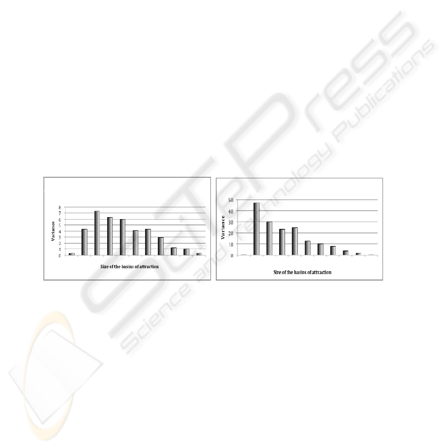
The according weight matrices were analyzed with respect to the variance of their
weight values. This variance analysis was separately performed for the weight matrix
between the input layer and the hidden layer and the matrix between the hidden layer
and the output one. The results are shown in figure 1:
Fig. 1. Variance of the first part of matrix (left figure) and the second part (right figure) in
relation to the size of the basins of attraction.
The order of the different networks in both figures is according to increasing size
of the basins of attraction. No 1 is the case with MC = 1:1, no 11 is the network with
MC = 1:11.
The left figure obviously gives no unambiguous result with respect to possible
relations between variance values and the size of basins of attraction but it suggest a
certain trend, namely the decreasing of the variance by increasing the basins sizes.
The right figure confirms this and even shows an unambiguous result: The variance
values indeed gradually decrease with the increasing of the size of the basins of
attraction. We then combined the two matrices by summing up the variance values of
both matrices and obtained the final result shown in figure 2:
0 1 3 4 5 6 7 8 9 10 11 0 1 3 4 5 6 7 8 9 10 11
17

Fig. 2. Variance and size of basins of attraction for the whole network; the networks are
ordered as in figure 1.
This final result completely confirms the trend shown in figure 1, left side, and the
clear results of figure 1, right side: the larger the size of the basins of attraction are,
i.e., the smaller the MC-values are, the smaller are the variance values and vice versa.
By the way, the difference between the variance of the upper matrix and that of the
lower one is probably due to the fact that the Back Propagation rule does not operate
in exactly the same way on both matrices: The lower half of the whole matrix is
changed by directly taking into account the error, i.e. the distance between the output
neurons and those of the target vector. The changing of the upper half of the matrix is
done by computing a certain proportion of the error and thus “dispersing” the changed
weight values with respect to those of the lower half. Yet these just force the variance
of the whole matrix to the shown result. If our networks had contained only two
layers the whole result would have been like that of figure 2. We shall come back to
this effect of a certain learning rule in the next section.
We did not expect such unambiguous results yet on hindsight they are quite
plausible and comprehensible: Low variance values mean dispersion of information
or of the differences between different information respectively because of the near
equality of the weight values. If on the other hand the weight values are significantly
different, i.e. a high variance, then differences between different messages can be
preserved. As small or large sizes respectively of basins of attraction have exactly that
effect on the performing of messages it is no wonder that we obtained that clear and
unambiguous relation between variance and size of basins of attraction.
Yet although these clear results are quite satisfactory we knew very well that they
must be treated with a great methodical caveat: the behaviour of neural networks, as
that of practically all complex dynamical systems, depends on many parameters, in
this case for example on specific propagation, activation and output functions, number
of layers, special learning rules and so on. The results shown above were obtained
with a specific type of neural network, although a standard and frequently used one
with a standard learning rule. To make sure that our results are not only valid for this
special methodical procedure we undertook another experimental series.
In these experiments we did not use one of the standard learning rules for neural
networks but a Genetic Algorithm (GA). The combination of a GA with neural
networks has frequently been done since the systematic analysis of neural networks in
the eighties. Usually a GA or another evolutionary algorithm is used in addition to a
certain learning rule in order to improve structural aspects of a network that are not
changed by the learning rule, e.g. number of layers, number of neurons in a particular
layer, threshold values and so on. In our experiments we used the GA as a substitute
0 1 3 4 5 6 7 8 9 10 11
18

for a learning rule like the Back Propagation rule in the first experimental series. The
according weight matrices of the different networks are, when using a GA, written as
a vector and the GA operates on these vectors by the usual “genetic operators”, i.e.
mutation and recombination (crossover).
We chose this procedure for two reasons: On the one hand the operational logic of
a GA or any other evolutionary algorithm is very different from that of the standard
learning rules. A learning rule modifies usually just one network; in this sense it is a
simulation of ontogenetic learning. In contrast an evolutionary algorithm always
operates on a certain population of objects and optimizes the single objects by
selecting the best ones from this population at time t. This is a model of phylogenetic
evolution. In addition learning rules like the Back Propagation rule or its simpler
form, namely the Delta Rule, represent the type of supervised learning. Evolutionary
algorithms represent another type of learning, i.e. the enforcing learning. In contrast
to supervised learning enforcing learning systems get no feed back in form of
numerical values that represent the size of the error. The systems just get the
information if new results after an optimization step are better or worse than the old
ones or if there is no change at all in the improvement process. Therefore, the training
procedure in the second series is as different from that of the first one as one can
imagine.
We assumed that by choosing such different procedures similar results from both
experiments would be a very strong indicator for our working hypothesis, namely the
relation between MC-values or size of the basins of attraction respectively and the
mentioned characteristics of the according weight matrices. To be sure, that would not
be a final proof but at least a “circumstantial evidence” that the results of the first
series are no artifacts, i.e., that they are not only effects from the chosen procedure.
On the other hand we were in addition interested in the question if networks with
certain MC-values are better or worse suited to adapt to changing environmental
conditions. It is evident that per se high or low MC-values are not good or bad. It
always depends on the situation if a network performs better with high or low
capabilities to generate different meanings. Sometimes it is better to process a
message in a rather general fashion and sometimes it is necessary to perceive even
small differences. Yet from a perspective of evolutionary adaptation it is quite
sensible to ask if systems with higher or lower MC can adjust better. That is why we
used an evolutionary algorithm to investigate this problem although it is another
question than that of a relation between the variance of the weight matrix and the
according MC-values.
Because a GA can be constructed with using many different parameters like size of
the mutation rate, size of the sub vectors in crossover, selection schemas, schemas of
crossover (“wedding schemas”), keeping the best “parents” or not and so on it is
rather difficult to obtain results that are representative for all possible GA-versions.
We used a standard GA with a mutation rate of 10%, a population of 20 networks,
initially generated at random, crossover segments of 5, and a selection schema
according to the fitness of the respective networks. Because the networks were
optimized with respect to the same association tasks as in the first series those
networks are “fitter” than others that successfully have learned more association tasks
than others. If for example a network is optimized with respect to the task to operate
according to two basins of attraction of size 8 then a network is better that correctly
19

associates 6 vectors of each basin to the target vector than a network that does this
only for 5 vectors.
The population consists again of three-layered feed forward networks with binary
coding for input and output layers; the input and output vectors consist of four
neurons and the hidden layer of three. As in the first series the networks operate with
the sigmoid activation function. We simplified the networks a bit because, as
mentioned, a GA has not one network to operate with but a whole population. The
target vectors were chosen at random; the vectors for the respective basins of
attraction were chosen according to their Hamming distance to those output vectors
that define the basins of attraction. It is no surprise that the GA came faster to
satisfactory results, i.e. the generation of networks that are able to solve the respective
association tasks, if the MC-values of the networks should be large than in the cases
when the MC should be small. The main results are shown in figure 3:
Fig. 3. Variance and size of basins of attraction in networks generated by a GA.
The figure obviously expresses a striking similarity to figure 1 of the first series.
The trend is the same, namely a clear relation between the size of the variance and the
increasing size of the basins of attraction or the decreasing size of the MC-values
respectively. Like in figure 1 the exceptions from this trend occur in the cases of
rather small basins of attraction, but only there. As we remarked in the preceding
section these exceptions may be due to the fact that the GA even more disperses the
weight values than does the Back Propagation rule for the upper half of the weight
matrix. This fact clearly demonstrates that the relation between variance values and
the sizes of the basins of attraction is “only” a statistical one, although the correlation
is very clear. We omit for the sake of brevity he results of the evolutionary analysis.
As we mentioned in the beginning of this section, the fact that such totally different
optimization algorithms like Back Propagation rule and GA, including the different
types of learning, generate the same trend with respect to our working hypothesis is
important evidence that the hypothesis may be valid in a general sense. Yet in both
series we just considered “case studies”, i.e. we concentrated in both cases on one
single network type and in the case of the GA-training on populations of the same
type of networks. That is why we started a third series.
3 Third Series: Statistical Analysis of Large Samples
Experiments with large samples of neural networks are always difficult because of the
large number of variables or parameters respectively that have to be taken into
20

account. Besides the influence of different learning rules, activation and propagation
functions and such parameters like learning rates and momentum the main problem is
a “combinatorial explosion”: if one takes into account the many different possible
combinations of neurons in the different layers and in addition the possible variations
of the number of layers one quickly gets such large samples that it is seldom possible
to obtain meaningful results. That is why we chose another way in the preceding
sections, namely the analysis of the two case studies in order to get a meaningful
hypothesis at all.
Yet despite the great difference between our two case studies it is always rather
problematic to draw general consequences from only several case studies. That is why
we studied a larger sample of two-layered neural nets, i.e., ca. 400.000 different
networks. We restricted the experiment to networks of two layers in order to keep the
experiments as clear as possible. The number of neurons in the input and output
vector are in all experiments the same and ranged from 3 to 10. The restriction to
equal dimensions of the two vectors was introduced because networks with different
sizes of the two vectors do not generate all MC-values with the same probability: If
the input vector is larger than the output one then MC = 1 would not be possible at all
because always more than one input vector will generate the same output vector. For
example, a simple network that is trained to learn a certain Boolean function has an
input vector of size 2 and an output vector of size 1. Its MC-value is 0.5. If conversely
the output vector is larger than the input vector the probability for large MC-values
will be greater than in networks with the same number of neurons in both vectors. To
avoid such distortions we used only vectors of equal size.
The networks were, as in the two case studies, binary coded and operated with the
sigmoid function. Thus we obtained ca. 400.000 pairs (MC, v), v being the variance.
The general results are the following:
As we supposed from the results of the two case studies the relation between
variance and MC-values is “only” a statistical one in the sense that there are always
exceptions from the general rule. Yet we discovered very clearly that indeed there is a
significant probability: the larger the variance is the smaller is the probability to
obtain networks with small MC-values, that is with large basins of attraction, and vice
versa. This result is in particular valid for variance values significantly large or small.
Only in the “middle regions” of variance values the probability to obtain MC-values
as a deviation from the general rule is a bit larger but not very much. This probability
distribution is shown in figure 4:
Fig. 4. Statistical relation between variance (x-axis) and MC-values (y-axis).
By the way, the deviations in the middle regions from the general trend may be a
first explanation for the mentioned results from section 2 with respect to the
1
1/n
21

evolutionary capability of networks with different MC-values. These networks adapt
more easily to changing environments than those with very large or very small values.
The hypothesis of the relation between MC-values and variance values seems to be
a valid one, at last as a statistical relation, Hence it is possible to predict the meaning
generating capacity of a network and thus its practical behaviour for certain purposes
with sufficient probability from a variance analysis of its weight matrix. Yet a caveat
is in order: We analyzed only one type of networks and further experiments are
necessary if our results are also valid for different types like, e.g. recurrent nets of
Self Organized Maps.
4 Interpretations and Conclusions
The behavior of complex dynamical systems can practically never be explained or
predicted by using only one numerical value (a scalar) as the decisive parameter. In a
mathematical sense the problem for such a system is always the task of solving
equations with a lot of variables, that is more variables than equations. It is well
known that for such tasks there is always more than one solution. When considering
neural networks by investigating the according weight matrix it is rather evident that
for example large basins of attraction may be constructed by very different matrices.
Hence, it is no wonder that the variance value, considered as a structural measure for
the occurrence of certain MC-values and the according sizes of the basins of
attraction, always allows for exceptions.
The knowledge about parameters that could predict the meaning generation
capacity would not only give important insights into the logic of neural network
operations; that would be an improvement of our theoretical understanding of these
complex dynamical systems. It could also give practical advantages if one needs
neural networks with certain capabilities – either if one needs robust networks with
great generalizing capacity or if there is need for sensitive networks that react in a
different manner to different inputs. To be sure, the relations we have discovered so
far are of only statistical validity. Yet to know that with a high probability one gets
the desired characteristics of a certain network if one constructs a weight matrix with
a specific variance is frequently a practical advantage: one has not to train the
networks and look afterwards if the network has the desired behavior but can
construct the desired matrix and if necessary make the additionally needed
improvements via learning rules and/or additional optimization algorithms like for
example a GA. For these theoretical and practical reasons it will be worthwhile to
investigate such relations as we have shown in this article further and deeper.
References
1. Klüver, J. and Klüver, C., 2007: On Communication. An Interdisciplinary and
Mathematical Approach. Dordrecht (NL): Springer.
2. Sacks, O., 1985: The Man Who Mistook His Wife for a Hat. New York: Summit Books.
3. Wolfram, S., 2001: A new Kind of Science. Champagne (Ill.): Wolfram Media.
22
