
FEATURE AND COMPUTATIONAL TIME REDUCTION ON
HAND BIOMETRIC SYSTEM
Carlos M. Travieso
1
, Jordi Solé-Casals
2
, Miguel A. Ferrer
1
and Jesús B. Alonso
1
1
Signals and Communication Department, Technological Centre for Innovation in Communnications
University of Las Palmas de Gran Canaria, Campus de Tafira, sn, Ed. de Telecomuncación
Pabellón B, Despacho 111, E35017, Las Palmas de Gran Canaria, Spain
2
Digital and Information Technologies Department, Digital Technologies Group, University of Vic
c/ de la Laura, 13, E-08500, Vic, Barcelona, Spain
Keywords: Principal Component Analysis, Pattern Recognition, Hand Biometric System, Parameterization, Feature
reduction, Classification system.
Abstract: In real-time biometric systems, computational time is a critical and important parameter. In order to improve
it, simpler systems are necessary but without loosing classification rates. In this present work, we explore
how to improve the characteristics of a hand biometric system by reducing the computational time. For this
task, neural network-multi layer Perceptron (NN-MLP) are used instead of original Hidden Markov Model
(HMM) system and classical Principal Component Analysis (PCA) procedure is combined with MLP in
order to obtain better results. As showed in the experiments, the new proposed PCA+MLP system achieves
same success rate while computational time is reduced from 247 seconds (HMM case) to 7.3 seconds.
1 INTRODUCTION
Biometrics is an emerging technology which is used
to identify or verify people by their physical or
behavioral characteristics. Amongst the physical
characteristics which have been used in biometrics
are the fingerprint, hand geometry, palm-print, face,
iris, retina, ear, etc. (Jain et al., 2001).
While systems based on fingerprint and eyes
features have, at least to date, achieved the best
matching performance, human hand provides the
source for a number of physiological biometric
features. The most frequently used are fingerprint,
palm-print, hand geometry, fingers geometry and
hand edge. These human hand features are relatively
stable and all the above mentioned characteristics
can be easily extracted from one single image of the
hand. Furthermore, these identification systems are
very well accepted by users, as are simples and do
not require to do anything special.
In this paper hand edge and its feature and time
computational reduction have been studied as a first
step for a real time application. We have worked on
a new parameterization for the hand edge, and after
the study of its behaviour, we have applied PCA
method in order to reduce the feature vector and
computational load of the system.
2 DATABASE
Our database has been built based on 60 users,
acquiring 10 samples per user. A scanner has been
used in order to acquire each sample. The following
table shows the most important characteristics of our
database.
Table 1: Characteristics of our database.
Parameters Data Example
Number of
classes
60
Number of
samples per
classes
10
Acquisition and
Quantification
Gray Scale (8
bits, 256 levels)
Resolution 150 dpi
Size
1403 x 1021
pixels
reduced to 80%
367
Travieso C., Solé-Casals J., Ferrer M. and Alonso J. (2010).
FEATURE AND COMPUTATIONAL TIME REDUCTION ON HAND BIOMETRIC SYSTEM.
In Proceedings of the Third International Conference on Bio-inspired Systems and Signal Processing, pages 367-372
DOI: 10.5220/0002591503670372
Copyright
c
SciTePress

3 PARAMETERIZATION
SYSTEM
We have considered just the hand perimeter. This
image is considered without the wrist that has been
extracted automatically from the shadow image.
Hands are scanned placed more or less on the center,
upward (wrist down).
Border determination as (x,y) positioning
perimeter pixels of black intensity, has been
achieved by processes of shadowing (black shape
over white background), filtering of isolated points,
and perimeter point to point continuous follow.
3.1 Perimeter Interpolation
Perimeter size variability induces us to consider a
convenient perimeter point interpolation, in order to
standardize perimeter vector description. For an
interpolating process, in order to achieve
reconstruction of the original shape, we may use any
of the well known algorithms as mentioned in (Fu
and Milios, 1994), (Loncaric, 1998), (Huang and
Cohen, 1996), but a simple control point’s choice
criterion in 1-D analysis allows for an appropriate
performance ratio on uniform control point’s
number and approximation error for all individuals
of all varieties studied.
The general idea, for such choice, is to consider
(x,y) positional perimeter points as (x,F(x)) graph
points of a 1-D relation F.
Consideration of y coordinate as y = F(x) is
done, because of the way, hands images are
presented in our study: hands have been scanned
with maximum size placed over x ordinate.
For a relation G to be considered as a one-
dimensional function, there is need to preserver a
correct sequencing definition (monotonic behavior).
That is: A graph,
)}(/),(,..1{
i
xf
i
y
i
y
i
xniG ===
(1)
It is the description of a function f if ordinate
points
nix
i
..1, = must be such that:
1..1,
1
−=<
+
nixx
ii
.
We consider then the border relation F as a union
of piece like curves (graphs) preserving the
monotonic behavior criterion, i.e.
∪
Jj
j
GF
∈
=
(2)
where:
JjFG
j
∈∀⊆ , and
}/),(,{
jjjj
fyyxJG
jjj
=
∈
=
ααα
α
,
For convenient sets of index J, J
j
and restriction
functions
}|{|
ji
j
Jxj
ff
∈
=
α
α
, such that the next point
following the last of G
j
is the first one of G
j
+1. G
j
graphs are correct f
j
functions descriptions.
Figure 1: Example of an F relation decomposed in graphs
with a correct function description.
Building the G
j
sets is a very straightforward
operation:
Beginning with a first point we include the next
one of F.
As soon as this point doesn’t preserve
monotonic behaviour we begin with a new Gj
+1.
Processes stop when all F points are assigned.
In order to avoid building G
j
reduced to
singletons, as show in figure 1 (G
4
and G
5
) the
original F relation may be simplified to preserve
only the first point of constant x ordinate series.
Afterwards, spreading of a constant number of
points is done proportional to the length of the G
j
and always setting in it is first one.
The point’s choice criterion mentioned before
allows, in two-dimensional interpolation, for taking
account on points where reverse direction changes
take place. Irregularity, of the surface curve, is
taken into account with a sufficient number of
interpolating points, as done in the uniform
spreading way.
The 1-D interpolation has been perform using
between 750 and 100 control points, with spline,
lineal or closest interpolated point neighborhood,
depending on the number of control points present
G
1
G
2
G
3
G
4
G
5
F = G
1∪
G
2∪
G
3∪
G
4∪
G
5
BIOSIGNALS 2010 - International Conference on Bio-inspired Systems and Signal Processing
368

in the decomposed curve. As a reference at 300 dpi a
crayon free hand trace is about 5 to 6 points wide.
Due to perimeter size variability inside a class,
coding of (x,y) control perimeter points have been
transformed taking account for size independence.
Considering the following definitions:
Γ the set of n, a fixed number, of control
points,
)},(/{
..1 iiini
yxXX ==Γ
=
Where (x
i
,y
i
) are
point coordinates of control perimeter points.
C
0
the central point of the
Γ
set:
),)(/1(
..1..1
0
∑∑
==
=
nini
ii
yxnC
,
/
Γ∈
= niii
yx
..1
),(
,
)(),(
1010 ++
==
iiiiii
XCXangleXXCangle
α
β
angles
defined for each interpolating points of
Γ .
Sequences of (x
i
,y
i
) positional points are then
transformed in sequence of
()
ii
β
ϕ
, angular points.
The choice of a starting and a central point
accounts for scale and leaf orientation. Placement of
both points sets the scale: its distance separation.
Relative point positioning sets the orientation of the
interpolating shape. Given a sequence of such angles
i
α
and
i
β
, it’s then possible to reconstruct the
interpolating shape of a leaf. Geometrical properties
of triangle similarities make such sequence size and
orientation free.
4 REDUCTION PARAMETERS
Principal Components Analysis (PCA) is a way of
identifying patterns in data, and expressing the data
in such a way as to highlight their similarities and
differences (Jolliffe, 2002). Since patterns in data
can be hard to find in data of high dimension, where
the luxury of graphical representation is not
available, PCA is a powerful tool for analyzing data.
The other main advantage of PCA is that once you
have found these patterns in the data, and you
compress the data, i.e. by reducing the number of
dimensions, without much loss of information.
PCA is an orthogonal linear transformation that
transforms the data to a new coordinate system such
that the greatest variance by any projection of the
data comes to lie on the first coordinate (called the
first principal component), the second greatest
variance on the second coordinate, and so on. PCA
is theoretically the optimum transform for a given
data in least square terms.
In PCA, the basis vectors are obtained by solving
the algebraic eigenvalue problem
(
)
TT
RXXR
=
Λ where X is a data matrix whose
columns are centered samples, R is a matrix of
eigenvectors, and
Λ
Γ
is the corresponding
diagonal matrix of eigenvalues. The projection of
data
XRC
T
nn
= , from the original p dimensional
space to a subspace spanned by n principal
eigenvectors is optimal in the mean squared error
sense.
Another possibility, not presented here, is to use
Independent Component Analysis (ICA) (Jutten and
Herault, 1991), (Hyvärinen et al. 2001) instead of
PCA. In this case, we obtain independent
coordinates and not only orthogonal as in previous
case. ICA has been used for dimensional reduction
and classification improvement with success
(Sanchez-Poblador et al., 2004).
In our problem we have 60 different classes of
hands, and for each class we have 10 different
samples, where each one is a two column matrix
between 750 and 100 points. First column
corresponds to interior angles
i
α
and second
column to exterior angles
i
β
, as explained before.
The procedure for applying PCA can be
summarized as follows:
1. Subtract the mean from each of the data
dimensions. This produces a data set whose
mean is zero (X).
2. Calculate de covariance matrix (Covx)
3. Calculate the eigenvectors e
i
and eigenvalues λ
i
of Covx
4. Order the eigenvectors e
i
by eigenvalue λ
i
,
highest to lowest. This gives us the components
in order of significance.
5. Form a feature vector by taking the eigenvectors
that we want to keep from the list of
eigenvectors, and forming a matrix (R) with
these eigenvectors in the columns.
6. Project the data to a subspace spanned by these
n principal components.
5 CLASSIFICATION SYSTEM
As classification system, two different models have
been used in this present work. Hidden Markov
Models (HMM), and Neural Networks (NN).
5.1 Hidden Markov Models
An HMM is the representation of a system in which,
for each value that takes a variable t, called time, it
FEATURE AND COMPUTATIONAL TIME REDUCTION ON HAND BIOMETRIC SYSTEM
369

is found in one and only one of N possible states and
declares a certain value at the output. Furthermore,
an HMM has two associated stochastic processes:
one hidden associate with the probability of
transition between states (non observable directly);
and another observable one, an associate with the
probability of obtaining each of the possible values
at the output, and this depends on the state in which
the system has been found (Rabiner and Juang,
1993). It has been used a Discrete HMM (DHMM),
which is defined by (Rabiner and Juang, 1993) and
(Rabiner, 1989);N is the number of states,
• M is the number of different observations,
• A(N,N) is the transition probabilities matrix
from one state to another,
• π(N,1) is the vector of probabilities that the
system begins in one state or another;
• and B(N,M) is the probabilities matrix for
each of the possible states of each of the
possible observations being produced.
We have worked with an HMM called "left to right"
or Bakis, which is particularly appropriate for
sequences. These “left to right” HMM’s turn out to
be especially appropriate for signature edge because
the transition through the states is produced in a
single direction, and therefore, it always advances
during the transition of its states. This provides for
this type of model the ability to keep a certain order
with respect to the observations produced where the
temporary distance among the most representative
changes. Finally, it has been worked from 40 to 80
states and 32 symbols per state.
In the DHMM approach, the conventional
technique for quantifying features is applied. For
each input vector, the quantifier takes the decision
about which is the most convenient value from the
information of the previous input vector. To avoid
taking a software decision, a fixed decision on the
value quantified is made. In order to expand the
possible values that the quantifier is going to
acquire, multi-labelling is used, so that the possible
quantified values are controlled by varying this
parameter. The number of labels in the DHMM is
related to values that can be taken from the number
of symbols per state.
DHMM algorithms should be generalized to be
adjusted to the output multi-labelling ({v
k
}k=1,..C),
to generate the output vector ({w(x
t
,v
k
)}k=1,..,C).
Therefore, for a given state j of DHMM, the
probability that a vector x
t
is observed in the instant
t, can be written as;
∑
=
=
C
k
jkttj
kbvxwxb
1
)(),()(
(3)
where b
j
(k) is the output discrete probability,
associated with the value v
k
and the state j; being C
the size of the vector values codebook.
5.2 Neural Networks
In recent years several classification systems have
been implemented using classifying techniques, such
as Neural Networks. The widely used Neural
Networks techniques are much known on
applications of pattern recognition.
The Perceptron of a simple layer establishes its
correspondence with a rule of discrimination
between classes, based on the lineal discriminator.
However, it is possible to define discriminations for
not lineally separable classes using multilayer
Perceptrons that are networks without refreshing
(feed-forward) with one or more layers of nodes
between the input layer and exit layer. These
additional layers contain hidden neurons or nodes,
are directly connected to the input and output layer
(Bishop, 1995).
A neural network multilayer perceptron (NN-
MLP) of three layers is shown on figure 2 and
implemented, with two layers of hidden neurons.
Each neuron is associated with weights and biases.
These weights and biases are set to each connections
of the network and, are obtained from training in
order to make their values suitable for the
classification task between the different classes. We
have used a back-propagation algorithm in order to
train the classification system.
Figure 2: Multilayer Perceptron.
BIOSIGNALS 2010 - International Conference on Bio-inspired Systems and Signal Processing
370
6 EXPERIMENTS AND RESULTS
All experiments have been repeated 5 fives or more,
therefore, the successes are showed by mean and
standard deviation. The first experiment was to find
the number of points more discriminate for the hand
edge. From 750 to 100 edge points were used, and
the best success was achieved with 200 points (see
table 2).
After this experiment, we begin to study the
feature reduction in order to keep the same success
rate. PCA method was used for this task.
Different number of components is considered in
the experiment, from 5 to 59 (as we have 60
different classes). As expected, the best
classification result was achieved with the maximum
number of principal components. Table 3
summarizes the success rates (only one experiment
for each case) obtained with different number of
principal components and using a multilayer
perceptron (MLP) as a classification system. The
neural network consisted of as many inputs as
principal components in the first layer, a hidden
layer of 60 nonlinear neurons (with tanh(·) as
activation function) and an output layer of 60
neurons. Scaled conjugate gradient was selected as
optimization algorithm, with a maximum of 500
epochs. Half of the examples where used for training
and the rest for test.
Table 2: Success rates for HMM classifier, using edge
information.
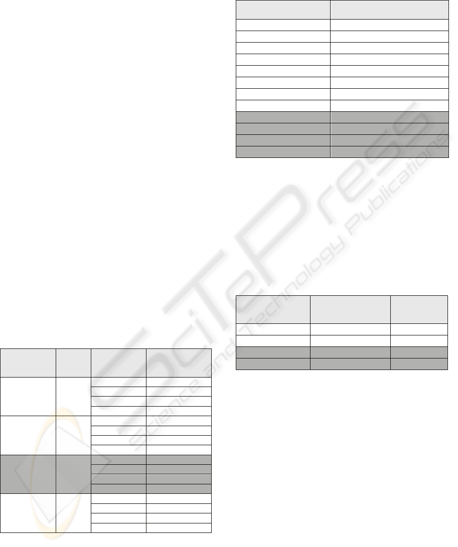
Table 3: Success rates for MLP classifier, using edge
information.
Number of
Principal Components
Success rates
5
46.00%
10
68.33%
15
75.00%
20
79.33%
25
78.33%
30
76.33%
35
78.00%
40
78.33%
45
78.67%
50
79.33%
55
79.33%
59
83.33%
In order to explore the performances of the
system, we repeat 20 times the classification
algorithm with MLP, for 20, 40 and 59 principal
components (see Table 4). Mean computational time
of the algorithm was also calculated, and for the
sake of comparison, we trained also a MLP with all
the available parameters without any PCA reduction
(corresponding to last line in Table 4).
Table 4: Success rates for MLP classifier, using edge
information.
Number of
Principal
Components
Success rates
Mean time
(seconds)
20
78.75% ± 0.81 7.30
40
80.93% ± 0.92 7.31
59
83.77% ± 1.34 7.30
398 features
83.60% ± 0.92 67.43
We can see that 59 components give us a success
rate as well as the HMM model while reducing the
standard deviation. On the other hand, if no PCA
algorithm is used, the system works well but the
computational time need for the system is higher (by
a factor of 10). For the HMM case, computational
time is much higher, about 247 seconds, and it can
be a problem in some real-time applications.
Taking all the results in consideration, in table 4
is shown that MLP can obtain similar results as
HMM (see table 2), and by using PCA, it has
dramatically been reduced the computational time,
as we deal with a much simpler classification
system. This point is crucial in real-time operating
systems and justifies the use of PCA+MLP
architecture instead of HMM solution.
Number of
edge points
HMM
states
Number of
samples
training
Success rates
750 60
4 46.61% ± 5.94
3 38.09% ± 4.73
2 32.41% ± 4.67
1 23.55% ± 3.73
300 60
4 72.50% ± 4.77
3 71.90% ± 4.36
2 61.04% ± 6.48
1 54.37% ± 5.71
200 60
4 84.17% ± 6.40
3 82.33% ± 4.33
2 79.79% ± 4.03
1 73.92% ± 5.64
100 60
4 73.12% ± 6.21
3 71.00% ± 7.84
2 70.33% ± 2.33
1 65.63% ± 5.63
FEATURE AND COMPUTATIONAL TIME REDUCTION ON HAND BIOMETRIC SYSTEM
371

7 CONCLUSIONS
In this work we have presented a PCA+MLP
architecture in order to classify 60 different classes
of hands that keeps the success rate achieved by a
HMM classification system, but with an important
improvement on the computational time reduction.
From HMM to MLP the computational time was
reduced by a factor of 33, and by using PCA we
have achieved to reduce 10 times more the
computational time. This is the first step to get this
application on real time, taking in account that the
implementation has been done in MATLAB
language.
Future work will include the study of
Independent Component analysis (ICA) as a feature
reduction dimension system in order to improve
success rates. Too, a verification system and a fusion
with geometry features will be implemented.
ACKNOWLEDGEMENTS
This work has been in part supported by “Programa
José Castillejo 2008” from Spanish Government
under the grant JC2008-00398; by the University of
Vic under de grant R0904; by private funds from
Spanish Company Telefónica, under “Cátedra
Teléfonica-ULPGC 2009”; and by funds from
Research Action from Excellent Networks on
Biomedicine and Environment belonging to
ULPGC.
REFERENCES
Jain., A., Bolle, R., Pankati, S., 2001. BIOMETRICS:
Personal Identification in Networked Society, Kluwer
Academic Press, 3
th
edition.
Lu, F. Milios, E.E., 1994. Optimal Spline Fitting to Planar
Shape, Elsevier Signal Processing No. 37- pp 129-140
S. Loncaric, S., 1998, A Survey of Shape Analysis
Techniques, Pattern Recognition. Vol 31 No. 8, pp.
983-1001
Huang, Z., Cohen, F., 1996, Affine-Invariant B-Spline
Moments for Curve Matching, IEEE Transactions on
Image Processing, Vol. 5. No. 10 , pp 824-836
Jolliffe I.T., 2002, Principal Component Analysis, Series:
Springer Series in Statistics, 2nd ed., Springer, NY
Jutten, C., Herault, J., 1991, Blind separation of sources,
Part 1: an adaptive algorithm based on neuromimetic
architecture, Signal Processing (Elsevier), Vol. 24 ,
Issue 1.
Hyvärinen, A., Karhunen, J., Oja, E., 2001, Independent
Component Analysis, New York, USA: John Wiley &
Sons
Sanchez-Poblador, V., Monte Moreno, E., Solé-Casals, J.,
2004. ICA as a preprocessing technique for
Classification”, ICA 2004, Granada, Spain. Lecture
Notes in Computer Science, Springer-Verlag Volume
3195/2004.
Rabiner, L., Juang, B.H., 1993. Fundamentals of Speech
Recognition. Ed. Prentice Hall
Rabiner, L.R., 1989. A tutorial on Hidden Markov models
and Selected Applications in Speech Recognition.
Proceedings of the IEEE. 77 (2), pp. 275-286
Bishop, C.M., 1995. Neural Networks for Pattern
Recognition. Ed. Oxford University Press.
BIOSIGNALS 2010 - International Conference on Bio-inspired Systems and Signal Processing
372
