ARALLEL CALCULATION OF

SUBGRAPH CENSUS IN BIOLOGICAL NETWORKS

Pedro Ribeiro, Fernando Silva and Lu

ıs Lopes

CRACS & INESC-Porto LA, Faculdade de Ci

encias, Universidade do Porto

Rua do Campo Alegre 1021, 4169-007 Porto, Portugal

Keywords:

Biological networks, Complex networks, Graph mining, Network motifs, Parallel algorithms.

Abstract:

Mining meaningful data from complex biological networks is a critical task in many areas of research. One

important example is calculating the frequency of all subgraphs of a certain size, also known as the sub-

graph census problem. This can provide a very comprehensive structural characterization of a network and

is also used as an intermediate step in the computation of network motifs, an important basic building block

of networks, that try to bridge the gap between structure and function. The subgraph census problem is com-

putationally hard and here we present several parallel strategies to solve this problem. Our initial strategies

were reﬁned towards achieving an efﬁcient and scalable adaptive parallel algorithm. This algorithm achieves

almost linear speedups up to 128 cores when applied to a representative set of biological networks from dif-

ferent domains and makes the calculation of census for larger subgraph sizes feasible.

1 INTRODUCTION

A broad range of biological structures can be rep-

resented as complex networks. The study of such

networks is relatively recent and has received in-

creased attention by the scientiﬁc community (Alm

and Arkin, 2003). A large number of concepts and

techniques appeared to analyze and understand com-

plex networks from any domain, leading to an impres-

sive panoply of different measurements used to mine

interesting data from them (Costa et al., 2007).

One important measure is the frequency in which

subgraphs appear in a network. Sometimes we are

just interested in determining frequent patterns (Ku-

ramochi and Karypis, 2001), while in others we need

to determine a full count of all different classes of iso-

morphic subgraphs (Bordino et al., 2008). This last

option is also known as a subgraph census and can

provide a very accurate structural characterization of

a network. This is typically applied for subgraphs of a

speciﬁc size and it is normally limited to small sizes,

mostly for efﬁciency reasons. This has been done

not only on biological networks (Middendorf et al.,

2004), but also on other domains, such as social net-

works analysis, where the triad census is very com-

mon (Wasserman et al., 1994).

Subgraph census also plays a major role as an in-

termediate step in the calculation of other important

measures, such as network motifs (Milo et al., 2002),

which are basically subgraphs that are statistically

over-represented in the network (and conjectured to

have some functional signiﬁcance). Network motifs

have applications on several biological domains, like

protein-protein interaction (Albert and Albert, 2004),

gene transcriptional regulation (Mazurie et al., 2005),

brain networks (Sporns and Kotter, 2004) and food

webs (Kondoh, 2008). Complex networks from other

domains can also be studied with motifs, like elec-

tronic circuits (Itzkovitz et al., 2005) or software ar-

chitecture (Valverde and Sol

e, 2005). The practi-

cal available algorithms and tools for network mo-

tifs all use a census to discover the frequency in the

original network and then calculate it again for a

series of similar randomized networks (Milo et al.,

2002; Wernicke, 2006). This is a computationally

hard problem that is closely related to the problem of

graph isomorphism (McKay, 1981). Some techniques

were developed to speedup the calculations, like sam-

pling (Kashtan et al., 2004), but they normally trade

accuracy for speed.

In all these applications, having a more efﬁcient

way to calculate the census is highly desirable. As

we increase the size of the subgraphs, their frequency

increases exponentially and it becomes unfeasible to

count all of them using traditional approaches. More-

over, to date, almost all algorithms for complete sub-

Ribeiro P., Silva F. and Lopes L. (2010).

PARALLEL CALCULATION OF SUBGRAPH CENSUS IN BIOLOGICAL NETWORKS.

In Proceedings of the First International Conference on Bioinformatics, pages 56-65

DOI: 10.5220/0002749600560065

 SciTePress

graph census are sequential. Some exceptions exist,

particularly in the area of network motifs, but they

are scarce and still limited (c.f. section 2.3). One rea-

son is that present network motifs methods still resort

to the generation of hundreds of random networks to

measure signiﬁcance. This puts the obvious opportu-

nity for parallelism not in the census itself but in the

generation of random networks and their respective

census. However, analytical methods to estimate the

signiﬁcance are now appearing (Matias et al., 2006;

Picard et al., 2008) and once they are fully developed

the burden of the calculation will then reside on the

census of the original network.

Considering the relevance of calculating exhaus-

tive census and the computational complexity in-

volved, resorting to parallel algorithms to speedup

the calculation is, in our view, an approach that will

impact in many application areas, particularly in the

study of biological networks. The use of parallelism

can not only speed up the calculation of census, but

also allow the calculation of the census for subgraph

sizes that were until now unreachable.

This paper focuses on strategies for solving the

subgraph census problem in parallel. With this ob-

jective in mind we start with an efﬁcient sequential

algorithm, ESU (Wernicke, 2006), and progressively

modify it to accommodate scalable parallel execution

and data-structures. This process led us to the for-

mulation of a novel adaptive parallel algorithm for

subgraph census that features a work sharing scheme

that dynamically adjusts to the available search-space.

The results obtained show that the algorithm is efﬁ-

cient and scalable.

The remainder of this paper is organized as fol-

lows. Section 2 establishes a network terminology,

formalizes the problem we want to tackle and gives an

overview of related work. Section 3 details all the fol-

lowed parallel strategies and the algorithm we devel-

oped. Section 4 discusses the results obtained when

applied to a set of representative biological networks.

Section 5 concludes the paper, commenting on the ob-

tained results and suggesting possible future work.

2 PRELIMINARIES

2.1 Network Terminology

In order to have a well deﬁned and coherent network

terminology throughout the paper, we ﬁrst review the

main concepts and introduce some notation that will

be used on the following sections.

A network can be modeled as a graph G com-

posed of the set V (G) of vertices or nodes and the

set E(G) of edges or connections. The size of a graph

is the number of vertices and is written as |V (G)|. A

k-graph is graph of size k. The neighborhood of a ver-

tex u ∈ V (G), denoted as N(u), is composed by the set

of vertices v ∈ V (G) that are adjacent to u (u is not in-

cluded). All vertices are assigned consecutive integer

numbers starting from 0, and the comparison v < u

means that the index of v is lower than that of u.

A subgraph G

of a graph G is a graph of size k

in which V (G

)⊆V (G) and E(G

)⊆E(G). This sub-

graph is said to be induced if for any pair of ver-

tices u and v of V (G

), (u, v) is an edge of G

and only if (u, v) is an edge of G. The neighborhood

of a subgraph G

, denoted by N(G

) is the union of

N(u) for all u ∈ V (G

). The exclusive neighborhood

of a vertex u relative to a subgraph G

is deﬁned as

excl

(u,G

) = {v ∈ N(u) : v /∈ G

∪ N(G

)}.

A mapping of a graph is a bijection where each

vertex is assigned a value. Two graphs G and H are

said to be isomorphic if there is a one-to-one map-

ping between the vertices of both graphs where two

vertices of G share an edge if and only if their corre-

sponding vertices in H also share an edge.

2.2 Subgraph Census

We give a rigorous deﬁnition for the subgraph census

problem:

Deﬁnition 1 (k-subgraph Census). A k-subgraph

census of a graph G is determined by the exact count

of all occurrences of isomorphic induced subgraph

classes of size k in G, where k ≤ |V (G)|.

Note that this deﬁnition is very broad and can be

applied to all kinds of networks, whether they are di-

rected or undirected, colored or not and weighted or

unweighted. Also note that here, unlike in (Kashtan

et al., 2004), we are concerned with an exact result

and not just an approximation.

A crucial concept that we have not yet completely

deﬁned is how to distinguish two different occur-

rences of a subgraph. Given that we are only inter-

ested in ﬁnding induced subgraphs, we can allow an

arbitrary overlap of vertices and edges or have some

constraints such as no edge or vertex sharing by two

occurrences. The several possibilities that we can

have for the frequency are considered and discussed

in (Schreiber and Schwobbermeyer, 2004). Here we

focus on the most widely used deﬁnition that we for-

malize next:

Deﬁnition 2 (Different occurences of k-subgraphs).

Two occurrences of subgraphs of size k, in a graph G,

are considered different if they have at least one vertex

PARALLEL CALCULATION OF SUBGRAPH CENSUS IN BIOLOGICAL NETWORKS

or edge that they do not share. All other vertices and

edges can overlap.

Note that this has a vital importance on the num-

ber of subgraphs we ﬁnd and consequently to the

tractability of the problem.

2.3 Related Work

There exists a vast amount of work on graph min-

ing. Particularly, the ﬁeld of frequent subgraph min-

ing has been very proliﬁc, producing sequential al-

gorithms like Gaston (Nijssen and Kok, 2004). Al-

though related, these algorithms differ substantially

in concept from our approach since their goal is to

ﬁnd the most frequent subgraphs that appear in a set

of graphs, while we try to ﬁnd the frequency of all

subgraphs on a single graph.

Regarding subgraph census itself, most of the

work on social networks is based on small sized sub-

graphs - mostly triads (Wasserman et al., 1994; Faust,

2007) - and therefore does not focus on efﬁciency, but

rather on the interpretation of the results. However,

for network motifs, efﬁciency does play an important

role and much importance is given to the algorithm for

generating the census. Increasing the speed may lead

to detection of bigger patterns and even an increase

in size of just one can yield scientiﬁcally important

results because a new previously unseen pattern with

functional signiﬁcance may be discovered.

The three best known production tools for ﬁnd-

ing motifs are all based on serial algorithms.

Mﬁnder (Milo et al., 2002) was the ﬁrst and it is based

on a recursive backtracking algorithm that generates

all k-subgraphs. It may generate the same subgraph

several times because it initiates a search procedure

in each of its nodes. Fanmod (Wernicke, 2006) uses

an improved algorithm called ESU, that only allows

searches being initiated on the nodes with an index

higher than the root node and therefore each subgraph

is found only once. MAVisto (Schreiber and Schwob-

bermeyer, 2004) does not improve efﬁciency except

when it uses a different concept for frequency.

Work on parallel algorithms for subgraph census

is scarce. Wang and Parthasarathy (2004) propose an

algorithm for ﬁnding frequent subgraphs but do not

count all of them. Schatz et al. (2008) focuses on net-

work motifs and how to parallelize queries of indi-

vidual subgraphs and not on how to enumerate all of

them.Wang et al. (2005) takes the closest approach to

our work. Their algorithm relies on ﬁnding a neigh-

borhood assignment for each node that avoids overlap

and redundancy on subgraph counts, as in Wernicke

(2006), and tries to statically balance the workload

“a priori” based only on each node degree (no details

are given on how this is done and how it scales). An-

other distinctive characteristic of their approach is that

they do not do isomorphism tests during the parallel

computation, they wait until the end to check all the

subgraphs and compute the corresponding isomorphic

classes. As we will see, our approach differs signif-

icantly from this one as it contributes with dynamic

and adaptive strategies for load balancing, thus attain-

ing higher efﬁciency.

3 PARALLEL ALGORITHMS

3.1 Core Sequential Unit

Given that we are interested in having an exact count

of all classes of isomorphic subgraphs, we must enu-

merate all subgraphs. The ESU algorithm (Wernicke,

2006) is a key component of the fastest network mo-

tif tool available and as far as we know it is one of

the most efﬁcient algorithms for subgraph enumera-

tion. Thus we chose the ESU algorithm as our starting

point and modiﬁed its recursive part to create a proce-

dure that given a graph G, a size k, a vertex minimum

index min, a partially constructed subgraph G

subgraph

and a list of possible extension nodes V

ext

, enumerates

all k-subgraphs that contain G

subgraph

and no nodes

with index lower than min. This procedure is depicted

in algorithm 1. It recursively extends the subgraph

subgraph

by ﬁrst adding the new node u. If the new

subgraph has size k, then it determines a unique iden-

tiﬁcation and saves it in a dictionary. Otherwise, it

expands the set of possible extension nodes, V

ext

, with

the nodes that are in the exclusive neighborhood of u

relative to the subgraph G

subgraph

and also satisfy the

property of being numerically bigger then min. If the

extension set of nodes is not null then a new node is

removed from extended V

ext

and recursion is made.

Algorithm 1 Extending a partially enumerated subgraph.

1: procedure EXTEND(G, k,min,u,G

subgraph

ext

)

2: G

subgraph

← G

subgraph

∪ {u}

3: if |V(G

subgraph

)| = k then

4: str ← CanonicalString(G

subgraph

)

5: Dictionary.AddAndIncrement(str)

6: else

7: V

ext

←V

ext

∪{v∈N

excl

(u,G

subgraph

) : v > min}

8: while V

ext

0 do

9: Remove an arbitrarily chosen v ∈ V

ext

10: Extend(G,k,min,v, G

subgraph

ext

)

Calling

Extend(

{}

)

for every u ∈

V (G) is exactly the equivalent to the original ESU al-

gorithm. Therefore, as long as we call it on all nodes,

BIOINFORMATICS 2010 - International Conference on Bioinformatics

we can be certain that it will produce complete results,

as shown in (Wernicke, 2006). Moreover,

Extend()

guarantees that each existent subgraph will only be

found once on the call of its lowest index, as exem-

pliﬁed in ﬁgure 1. This avoids redundant calculations

as in (Wang et al., 2005) and is crucial to achieve an

efﬁcient census.

Figure 1: Example of how

Extend()

calls generate all sub-

graphs.

Before going into the details of the parallelism

two additional notes are needed. First, isomorphism

(line 4 of the procedure) is taken care of by using the

canonical string representation of the graphs, deﬁned

as the concatenation of the elements of the adjacency

matrix of the canonical labeling. In our case we use

McKay’s nauty algorithm (McKay, 1981), a widely

known fast and practical implementation of isomor-

phism detection. Second, in order to store the results

found within one call to our procedure (line 5), we

use a string dictionary structure. This can be imple-

mented in many ways, for example using an hash ta-

ble or a balanced red-black tree. We implement the

later (using STL map from C++).

3.2 Initial Parallel Approaches

Each of the aforementioned calls to

Extend(

{}

)

is completely inde-

pendent from each other and we call it a primary

work unit. A possible way of parallelizing subgraph

census is then to distribute these work units among

all CPUs

. The problem is that these units have

a computational cost with a huge variance, as the

inherent substructure and the number of subgraphs

each one enumerates are also quite different.

We experimented several strategies for the distri-

bution in order to obtain the desired load balance. The

ﬁrst one was to statically allocate the units to workers

before starting the census computation. In order to

obtain good results this would need accurate estimates

of the time that each unit takes to compute. We were

unable to do that with the desired accuracy, since cal-

from now on we will refer to processors in computa-

tional nodes as CPUs or workers to avoid confusion be-

tween them and graph nodes.

culating this is almost as difﬁcult as enumerating the

subgraphs themselves.

We then took the path of a more dynamic ap-

proach using a master-worker architecture (Heymann

et al., 2000). The master maintains a list of unpro-

cessed primary work units. Workers ask the master

for a unit, process it and repeat until there is noth-

ing more to compute. Each worker maintains its own

dictionary of frequencies. When all work units have

been computed the master is responsible for collect-

ing and merging all results, summing up the frequen-

cies found.

The position of the work units on the master’s list

will determine the total time needed and we tried sev-

eral strategies. Initially we just added all work units

to the list in chronological order of the nodes. This

proved to be a bad strategy since it is the same as a

random assignment, which is in principle the worst

possible (Heymann et al., 2000). We then experi-

mented giving the work units sorted to an estimated

cost, using LPTF (Largest Processing Time First)

strategy. If the estimate was perfect, it is known that

we would achieve at least

of the optimum (Hall,

1997). We only had an approximation (based on

the number of nodes achievable in k − 1 steps) and

therefore that boundary is not guaranteed. However,

since our heuristic function maintained a reasonable

ordering of the nodes, the performance was vastly im-

proved.

We still had the problem that the call to a few

primary work units (potentially even just one) could

consume almost all the necessary compute time. This

prevents good load balance strategies, given that each

work units runs sequentially. This problems occurs

very often in reality because typical complex net-

works are scale free (Barabasi and Albert, 1999).

Whenever their hubs are the starting nodes of a work

unit, very large neighborhoods are induced and a huge

amount of subgraphs is generated. No matter what

we do, there will always be a worker computing the

largest sequential work unit and therefore the total

compute time needed cannot be smaller than that.

On some of our experiments with real biological net-

works, this largest atomic unit could consume more

than 25% of the total execution time, which limits our

scalability.

Considering that a work unit only calculates sub-

graphs containing nodes with indices greater than the

index of the initial node, we devised a novel strategy

in which we give higher index numbers to the poten-

tially more time consuming nodes (those with larger

degrees). We expected this to reduce the number of

subgraphs spawning from these nodes, thus reducing

the granularity of the work units induced by those

PARALLEL CALCULATION OF SUBGRAPH CENSUS IN BIOLOGICAL NETWORKS

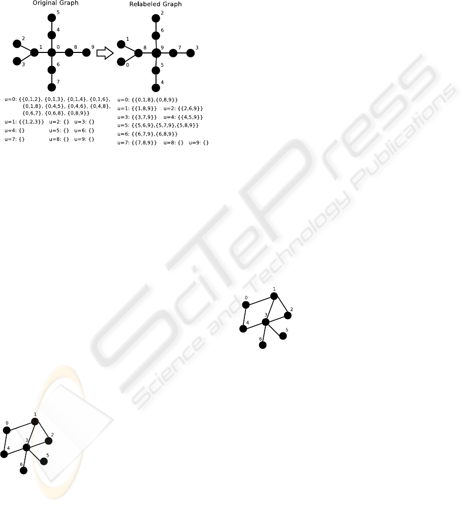
nodes. To accomplish this strategy, we implemented

a node relabeling algorithm in which the nodes are

sorted increasingly by their degree. Figure 2 gives a

practical example of this strategy at work, producing

a more balanced graph.

Figure 2: Relabeling the graph to balance primary work

units.

Although this last approach improved our results,

we expected that for some networks the relabeling

strategy could not reduce enough the granularity of

the work units, thus preventing scalability. We felt

that we really needed a strategy that could divide the

work units further.

3.3 Adaptive Parallel Enumeration

By inspecting the computation ﬂow of a primary work

unit, we can observe that there are several recursive

calls to

Extend()

, as exempliﬁed in ﬁgure 3 (for sim-

plicity, we do not show G and k since these are ﬁxed

arguments).

Extend(

{}

)

ext

= {1,4}

Extend(

{0}

{4}

)

ext

= {2,3,4}

Extend(

{0,1}

{3,4}

)

→ Found subgraph {0,1,2}

Extend(

{0,1}

{4}

)

→ Found subgraph {0,1,3}

Extend(

{0,1}

{}

)

→ Found subgraph 0,1,4

Extend(

{0}

{}

)

ext

= {3}

Extend(

{0,4}

{}

)

→ Found subgraph 0,3,4

Figure 3: The computation ﬂow of a primary work unit.

With our formulation of

Extend()

, all recursive

calls are independent with no need for information of

previous data on the recursion stack besides the argu-

ments it was called with. One way to divide a primary

work unit is therefore to partitionate it in its recursive

calls. A tuple (min, u,G

subgraph

ext

) completely de-

ﬁnes the resulting call to

Extend()

and we will now

call work unit to a tuple like this, with primary work

units being only a particular case.

Our new strategy to reduce the granularity of the

work units uses a threshold parameter to indicate the

point in the computation at which we split the ex-

ecution of the current work unit into smaller work

units. Instead of really computing subsequent recur-

sive calls, we encapsulate their arguments into new

smaller work units and send them to the master to be

added to the list of unprocessed work, effectively di-

viding our previously atomic sequential units. This

leads to a simpler, yet elegant, solution when com-

pared to more common adaptive strategies that need a

queue in each computation node (Eager et al., 1986).

Figure 4 illustrates our strategy at work. Remem-

ber that the new work units are still independent and

we do not need to be concerned with locality. All

subgraphs will be found and added to the respective

worker’s dictionary of frequencies, being merged in

the end of the whole computation to determine the

global resulting census.

Extend(

{}

)

ext

= {1,4}

Extend(

{0}

{4}

)

ext

= {2,3,4}

Extend(

{0,1}

{3,4}

)

→ Found subgraph {0,1,2}

——– Splitting Threshold ——–

Extend(

{0,1}

{4}

)

⇒ New work unit with these arguments

Extend(

{0,1}

{}

)

⇒ New work unit with these arguments

Extend(

{0}

{}

)

⇒ New work unit with these arguments

Figure 4: Work split strategy for work units.

Our algorithm is able to adjust itself during exe-

cution using this division strategy. It splits large work

units into new smaller work units ensuring that their

grain-size will never be larger than the size of work

units executed up to the threshold value. In doing so,

we are able to improve the load balancing and thus

achieve an effective dynamic and adaptive behavior.

The splitting threshold parameter is central in our

adaptive algorithm. If it is set too high, the work units

will not be sufﬁciently divided in order to adequately

balance the work among all CPUs. If it is too low,

work will be divided too soon and the communication

costs will increase. As a proof of concept our cur-

BIOINFORMATICS 2010 - International Conference on Bioinformatics

rent implementation uses a threshold that limits the

computation time spent on a work unit to a maximum

value, but other measures could be used like for ex-

ample the number of subgraphs already enumerated.

One aspect not yet discussed, but that is orthogo-

nal to all discussed strategies, concerns the aggrega-

tion of results at the master. If a naive approach was

taken, then each worker would be sending their results

to the master sequentially. This would be highly in-

efﬁcient and therefore we devised a parallel approach

for this ﬁnal step. We use an hierarchical binary tree

to organize the aggregation of results, where each

worker receives the results of two other child workers,

updates its own frequency dictionary accordingly, and

then in turn sends the aggregated results to its parent.

This is exempliﬁed in ﬁgure 5 and has the potential

to logarithmically reduce the total time needed to ac-

complish this step.

Figure 5: Example of results aggregation with 1 master and

6 workers.

All the ideas described are the basis for our main

algorithm that we called Adaptive Parallel Enumera-

tion (APE). Algorithms 2 and 3 describe in detail our

APE master and worker procedures.

Algorithm 2 APE master node.

1: procedure MASTER(G,k)

2: L

WorkUnits

.add(AllPrimaryWorkUnits)

3: while CPUsWorking 6=

0 do

4: msg ← ReceiveMessage(AnyWorker)

5: if msg.type = RequestForWork then

6: if L

WorkUnits

.notEmpty() then

7: W ← L

WorkUnits

.pop()

8: newMsg ← EncapsulateWorkUnit(W )

9: SendMessage(msg.Sender,newMsg)

10: else

11: IdleWorkers.push(msg.Sender)

12: else if msg.type = NewWorkUnit then

13: if IdleWorkers.notEmpty() then

14: worker ← IdleWorker.pop()

15: SendMessage(worker,msg)

16: else

17: W ← ExtractWorkUnit(msg)

18: L

WorkUnits

.push(W)

19: BroadcastMessage(Terminate);

20: ReceiveResults(Le f tChild,RightChild)

The master starts by adding all primary work units

to the list of unprocessed work units (L

WorkUnits

Then starts its main cycle where it waits for a mes-

sage from a worker. If the message indicates that the

worker needs more work, the master sends it the next

unprocessed work unit L

WorkUnits

. If the list is empty,

the master signals the worker as being idle. If the mes-

sage indicates that the worker is splitting work and

thus sending a new unprocessed work unit, then the

master adds that new work unit to L

WorkUnits

. If there

is an idle worker, then this unit is sent right away to

that worker. When all workers are idle, the subgraph

enumeration is complete and the master ends its main

cycle, broadcasting to all workers that event. What

remains is then to collect the results and following the

explained hierarchical aggregation process, the mas-

ter receives the results of two workers and merges

them in an uniﬁed global dictionary of the frequen-

cies of each isomorphic class of k-subgraphs.

Algorithm 3 APE worker node.

1: procedure WORKER(G,k)

2: while msg.type 6= Terminate do

3: msg ← ReceiveMessage(Master)

4: if msg.type = NewWorkUnit then

5: W = (G, k, min, u,G

subgraph

ext

) ←

ExtractWorkUnit(msg)

6: Extend’(W)

7: ReceiveResults(Le f tChild,RightChild)

8: SendResults(ParentWorker)

9: procedure EXTEND’(W)

10: if SplittingThresholdAchieved() then

11: msg ← EncapsulateWorkUnit(W)

12: SendMessage(Master,msg)

13: else

14: lines 2 to 9 of algorithm 1

15: Extend’(W

= (G,k, min,v, G

subgraph

ext

))

16: lines 11 and 12 of algorithm 1

The worker has a main cycle where it waits for

messages from the master. If the message signals a

new work unit to be processed, than it calls a mod-

iﬁed version of the

Extend()

procedure to compute

that work unit. If the message signals termination,

then it exits the cycle, receiving and merging the re-

sults from two other workers with its own dictionary.

It then send those results to a single parent processor,

that depending on the worker rank number may be

other worker or the master itself, completing the hi-

erarchical aggregation phase. Regarding the modiﬁed

version of the

Extend()

procedure, it is exactly the

same as the version depicted on algorithm 1 except

the fact than when the splitting threshold is achieved,

the computation is stopped and all subsequent calls

consist now in encapsulating the arguments into a new

work unit and sending it to the master.

There are two issues that we would like to clarify.

PARALLEL CALCULATION OF SUBGRAPH CENSUS IN BIOLOGICAL NETWORKS

Table 1: Networks used for experimental testing of the algorithms.

Network Nodes Edges Avg. Degree Description

Neural

297 2345 7.90 Neural network of C. elegans

Gene

688 1079 1.57 Gene regulation network of S. cerevisiae

Metabolic

1057 2527 2.39 Metabolic network of S. pneumoniae

Protein

2361 7182 3.04 Protein-protein interaction network of S. cerevisiae

First, we decided to use a dedicated master because

it is a central piece in the architecture and we needed

the highest possible throughput in the assignment of

new work units to idle workers. Second, APE was

originally created having in mind homogeneous re-

sources but its dynamic and adaptive design makes it

also suited for heterogeneous environments.

4 RESULTS

All experimental results were obtained on a dedicated

cluster with 12 SuperMicro Twinview Servers for a

total of 24 nodes. Each node has 2 quad core Xeon

5335 processors and 12 GB of RAM, totaling 192

cores, 288 GB of RAM, and 3.8TB of disk space, us-

ing Inﬁniband interconnect. The code was developed

in C++ and compiled with gcc 4.1.2. For message

passing we used OpenMPI 1.2.7. All the times mea-

sured were wall clock times meaning real time from

the start to the end of all processes.

In order to evaluate our parallel algorithms we

used four different representative biological networks

from different domains:

Neural

(Watts and Strogatz,

1998),

Gene

(Milo et al., 2002),

Metabolic

(Jeong

et al., 2000) and

Protein

(Bu et al., 2003). The

networks present varied topological features that are

summarized in Table 1.

We ﬁrst studied the computational behaviour of

each network using the equivalent to the ESU al-

gorithm, sequentially calling all primary work units

(with no MPI overhead). This measures how much

time a serial program would take to calculate a sub-

graph census. We took note of what was the maxi-

mum possible subgraph size k achievable in a reason-

able amount of time (we chose one hour as the max-

imum time limit). We calculated the average growth

ratio, that is, by which factor did the execution time

grew up as we increased k by one. Finally, we also

calculated the total number of different occurrences

of k-subgraphs and the number of different classes of

isomorphism found on those subgraphs. The results

obtained can be seen in table 2.

Note the relatively small subgraph sizes achiev-

able. This is not caused by our implementation, since

using the FANMOD tool (Wernicke, 2006), the fastest

Table 2: Maximum achievable subgraph sizes k using a se-

rial program.

Network k

Time Average Total nr of Isomor.

spent (s) Growth subgraphs classes

Neural

6 10,982.9 47.6±0.4 1.3 × 10

286,376

Gene

7 4,951.0 19.0±1.4 4.2 × 10

4,089

Metabolic

6 14,000.1 46.5±2.7 1.9 × 10

1,696

Protein

6 10,055.2 31.2±3.1 1.3 × 10

231,620

available for network motifs calculation, we also were

only able to achieve the same maximum k in one hour.

The cause is that, as expected, the computing time

grows exponentially as the subgraph size increases.

We also observe that although different graphs present

very different average growths, the growth rate for a

given graph seems fairly constant (note the standard

deviation).

For the next set of results we decided to ﬁx the

respective k for each graph to the values depicted in

table 2, in order to have more comparable results.

We evaluated the parallel strategies described in sec-

tion 3. We compared the speedup obtained on all

three graphs for the dynamic strategy with chrono-

logical order in the work units list (DYN-CRON),

with LPTF ordering (DYN-LPTF), with graph rela-

beling followed by LPTF (DYN-RELABEL) and ﬁ-

nally with the APE strategy.

For the APE algorithm it is necessary to explain

how we chose the value for the splitting threshold pa-

rameter. We chose to employ the time spent in the

same work unit as a proof of concept for the useful-

ness of APE and we empirically experimented several

values for this time limit, reducing it while verifying

that the speedup was being improved. This value con-

trols the granularity of the work units. We want it as

small as possible, as long as the increase in communi-

cation costs does not overcome the effect of increased

sharing. We found that for our context 2 seconds ap-

peared to be a good and balanced value (the time spent

in communications during the enumeration of the sub-

graphs was always smaller than 2% of the total time

spent), and we measured the speedup with that partic-

ular value chosen as the threshold (APE-2s).

We used a minimum of 8 CPUs because each com-

putation node in the cluster had precisely that number

of processors. With less CPUs the nodes would not

BIOINFORMATICS 2010 - International Conference on Bioinformatics

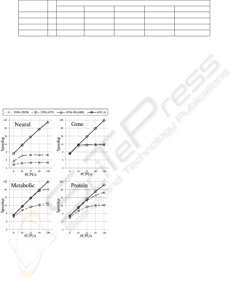
Table 3: Detailed APE behavior with splitting threshold set to 2s.

Network k

#CPUs: speedup (% time spent in aggregating results)

8 16 32 64 128

Neural

6 7.0 (0.2%) 14.8 (1.2%) 30.1 (3.4%) 58.7 (8.0%) 107.0 (16.9%)

Gene

7 7.0 (0.1%) 15.0 (0.2%) 30.7 (0.4%) 62.0 (0.8%) 125.0 (0.7%)

Metabolic

6 6.9 (0.1%) 14.9 (0.1%) 30.8 (0.3%) 62.4 (0.6%) 125.5 (1.3%)

Protein

6 6.6 (0.2%) 13.7 (1.2%) 28.0 (3.3%) 54.6 (7.4%) 96.9 (18.8%)

be exclusively dedicated to the subgraph census. The

results obtained up to 128 processors are depicted in

ﬁgure 6. The results obtained clearly show different

performance levels for the different strategies. Gener-

ally speaking, the strategies based on the atomic pri-

mary work units do not scale well, although the in-

cremental strategies used show some improvements

in the speedup. Overall, as expected, the adaptive

strategy, APE-2s, outperforms all others and clearly

achieves scalability.

Figure 6: Speedups obtained with several parallel ap-

proaches.

Next, we further analyze the performance of APE-

2s on all networks. Table 3 details the performance of

the APE-2s up to 128 processors, and show the per-

centage of time spent in the ﬁnal step of aggregating

all frequency results in the master CPU.

We can observe that for

Gene

and

Metabolic

APE-2s obtains almost perfect linear speedup, with

a reduced amount of time spent in the aggregation

phase. In

Neural

and

Protein

, despite the good re-

sults, there is still some room for improvement. The

time spent communicating the results in the end of the

computation, more than 15% of the execution time

with 128 processors, is the cause for the loss in the

speedup. In fact, with more than 200,000 classes of

isomorphic subgraphs in the network (see table 2),

each worker has to communicate all of the frequen-

cies it ﬁnds in its respective computation. On aver-

age, the number of different classes of isomorphism

discovered on the same CPU, is larger than 150,000.

Each of these classes has to be encapsulated (uniquely

identifying the class) in order for the receiver to be

able to decode it and merge the results. Even with our

hierarchical method for aggregating the results, this

still takes a considerable amount of time. This effect

is not so noticeable in the other networks since the

number of different classes found is much lower (due

to inherent network topology, with a smaller average

degree per node).

As a ﬁnal demonstration of the relevance of our al-

gorithm, consider the average growth as we increase

k (shown in Table 2). As long as the number of pro-

cessors we have available is larger than the average

growth, we should be able to compute the (k + 1)-

census in the same amount of time we initially were

able to compute the k-census sequentially. For exam-

ple, using the average growth, we can estimate that

calculating a 7-census of

Metabolic

would take more

than one week, if done sequentially. Using 128 pro-

cessors and APE-2s, we were able to calculate it in

less than 1h30m, spending even less than half of the

time a sequential 6-census takes.

5 CONCLUSIONS

We presented several strategies for calculating sub-

graph census of biological networks in parallel. Our

approaches are based on an efﬁcient sequential al-

gorithm called ESU that we parallelized by initially

modifying it to a version capable of producing inde-

pendent and dividable work units. We started with

a dynamic master-worker strategy and subsequently

improved it with an LPTF order of processing and a

smart relabeling of the nodes in the graph. We also

PARALLEL CALCULATION OF SUBGRAPH CENSUS IN BIOLOGICAL NETWORKS

presented APE, a novel adaptive load balancing al-

gorithm, which includes an hierarchical aggregation

of the results found in each worker. APE proved to

be an acceptable and scalable solution for the set of

representative networks studied, successfully reduc-

ing the time needed to calculate the subgraph census

and achieving larger subgraph sizes than were before

possible.

The main drawback of APE seems to be the ﬁ-

nal aggregation of results. We plan to research and

improve this step in the future. One way of doing it

would be to use a more compact and compressed rep-

resentation of the results. We also plan to research

the splitting threshold parameter in order to better un-

derstand on what does it depend, exactly how does it

affect the computation and how could it be automati-

cally determined by the algorithm. We are collaborat-

ing with neuroinformatics scientists in order to apply

the described strategies on real neural networks to ob-

tain new and interesting results on previously unfea-

sible subgraph census.

ACKNOWLEDGEMENTS

We thank Enrico Pontelli for the use of Inter Clus-

ter in the New Mexico State University. Pe-

dro Ribeiro is funded by an FCT Research Grant

(SFRH/BD/19753/2004). This work was also par-

tially supported by project CALLAS of the FCT (con-

tract PTDC/EIA/71462/2006).

REFERENCES

Albert, I. and Albert, R. (2004). Conserved network mo-

tifs allow protein-protein interaction prediction. Bioin-

formatics, 20(18):3346–3352.

Alm, E. and Arkin, A. P. (2003). Biological networks. Cur-

rent Opinion in Structural Biology, 13(2):193–202.

Barabasi, A. L. and Albert, R. (1999). Emergence of scaling

in random networks. Science, 286(5439):509–512.

Bordino, I., Donato, D., Gionis, A., and Leonardi, S.

(2008). Mining large networks with subgraph counting.

In Procs of the 8th IEEE International Conference on

Data Mining (ICDM), pages 6 pp.+.

Bu, D., Zhao, Y., Cai, L., Xue, H., Zhu, X., Lu, H., Zhang,

J., Sun, S., Ling, L., Zhang, N., Li, G., and Chen, R.

(2003). Topological structure analysis of the protein-

protein interaction network in budding yeast. Nucl. Acids

Res., 31(9):2443–2450.

Costa, L., Rodrigues, F. A., Travieso, G., and Boas, P. R. V.

(2007). Characterization of complex networks: A survey

of measurements. Advances In Physics, 56:167.

Eager, D. L., Lazowska, E. D., and Zahorjan, J. (1986).

Adaptive load sharing in homogeneous distributed sys-

tems. IEEE Trans. Softw. Eng., 12(5):662–675.

Faust, K. (2007). Very local structure in social networks.

Sociological Methodology, 37(1):209–256.

Hall, L. A. (1997). Approximation algorithms for schedul-

ing. In Approximation algorithms for NP-hard problems,

pages 1–45, Boston, MA, USA. PWS Publishing Co.

Heymann, E., Senar, M. A., Luque, E., , and Livny, M.

(2000). Evaluation of an adaptive scheduling strategy

for master-worker applications on clusters of worksta-

tions. In Proc. of the 7th International Conference on

High Performance Computing, Bangalore, India.

Itzkovitz, S., Levitt, R., Kashtan, N., Milo, R., Itzkovitz,

M., and Alon, U. (2005). Coarse-graining and self-

dissimilarity of complex networks. Phys Rev E Stat Non-

lin Soft Matter Phys, 71(1 Pt 2).

Jeong, H., Tombor, B., Albert, R., Oltvai, Z. N., and

Barab

asi, A. L. (2000). The large-scale organization of

metabolic networks. Nature, 407(6804):651–654.

Kashtan, N., Itzkovitz, S., Milo, R., and Alon, U. (2004).

Efﬁcient sampling algorithm for estimating subgraph

concentrations and detecting network motifs. Bioinfor-

matics, 20(11):1746–1758.

Kondoh, M. (2008). Building trophic modules into a per-

sistent food web. Proceedings of the National Academy

of Sciences, 105(43):16631–16635.

Kuramochi, M. and Karypis, G. (2001). Frequent subgraph

discovery. IEEE International Conference on Data Min-

ing, 0:313.

Matias, C., Schbath, S., Birmel, E., Daudin, J.-J., and

Robin, S. (2006). Network motifs: mean and variance

for the count. REVSTAT, 4:31–35.

Mazurie, A., Bottani, S., and Vergassola, M. (2005). An

evolutionary and functional assessment of regulatory net-

work motifs. Genome Biology, 6:R35.

McKay, B. (1981). Practical graph isomorphism. Congres-

sus Numerantium, 30:45–87.

Middendorf, M., Ziv, E., and Wiggins, C. (2004). Infer-

ring network mechanisms: The drosophila melanogaster

protein interaction network. PNAS, 102:3192.

Milo, R., Shen-Orr, S., Itzkovitz, S., Kashtan, N.,

Chklovskii, D., and Alon, U. (2002). Network motifs:

simple building blocks of complex networks. Science,

298(5594):824–827.

Nijssen, S. and Kok, J. N. (2004). Frequent graph mining

and its application to molecular databases. In SMC (5),

pages 4571–4577. IEEE.

Picard, F., Daudin, J.-J. J., Koskas, M., Schbath, S., and

Robin, S. (2008). Assessing the exceptionality of net-

work motifs. J Comput Biol.

Schatz, M., Cooper-Balis, E., and Bazinet, A. (2008). Par-

allel network motif ﬁnding.

Schreiber, F. and Schwobbermeyer, H. (2004). Towards mo-

tif detection in networks: Frequency concepts and ﬂexi-

ble search. In Proceedings of the International Workshop

on Network Tools and Applications in Biology (NET-

TAB04, pages 91–102.

BIOINFORMATICS 2010 - International Conference on Bioinformatics

Sporns, O. and Kotter, R. (2004). Motifs in brain networks.

PLoS Biology, 2.

Valverde, S. and Sol

e, R. V. (2005). Network motifs in com-

putational graphs: A case study in software architecture.

Physical Review E (Statistical, Nonlinear, and Soft Mat-

ter Physics), 72(2).

Wang, C. and Parthasarathy, S. (2004). Parallel algorithms

for mining frequent structural motifs in scientiﬁc data.

In In ACM International Conference on Supercomputing

(ICS) 2004.

Wang, T., Touchman, J. W., Zhang, W., Suh, E. B., and Xue,

G. (2005). A parallel algorithm for extracting transcrip-

tion regulatory network motifs. Bioinformatic and Bio-

engineering, IEEE International Symposium on, 0:193–

200.

Wasserman, S., Faust, K., and Iacobucci, D. (1994). Social

Network Analysis : Methods and Applications (Struc-

tural Analysis in the Social Sciences). Cambridge Uni-

versity Press.

Watts, D. J. and Strogatz, S. H. (1998). Collective dynamics

of ’small-world’ networks. Nature, 393(6684):440–442.

Wernicke, S. (2006). Efﬁcient detection of network mo-

tifs. IEEE/ACM Trans. Comput. Biol. Bioinformatics,

3(4):347–359.

PARALLEL CALCULATION OF SUBGRAPH CENSUS IN BIOLOGICAL NETWORKS