PRACTICAL EDUCATION OF CONTROL ENGINEERING
Using Open OS, Free Software and Actual Plant
Sunao Tanimoto, Kiyoshi Yoshida
Nippon Institute of Technology, Miyashiro, Minami-Saitama, Saitama, 345-8501, Japan
Jyunichiro Tahara
Japan Agency for Marine-Earth Science and Technology (JAMSTEC), Japan
Keywords: Experiment Devices, Computer Control, Modern Control Theory, Plant Control, Linux, Octave, Control
CAD.
Abstract: The importance to educate control engineers is to make them experience the modern control theory by the
actual devices instead of pure digital simulator. During these applications, students will face to every
existing problem and digest the fruits of control theory by tangible impression. This paper reports the
development of experiment devices for computer control engineering education, where a pendulum is
controlled by a General Linux P/C through a DC motor every 1ms, realizing most kinds of advanced control
schemes linked with free control CAD, Octave. Controlled examples with various schemes are reported.
1 INTRODUCTION
Control engineering has an important role in
industries. Authors feel that the education for control
engineers has the problem that it mainly depends on
just the computer simulations. This seldom offers
tangible advanced control experiences to engineers
or students, and valuable theories are not applied to
actual fields well. To cope with this problem,
authors developed actual motor driven
pendulum/arm real-time control experimental
systems with an open source code OS; Linux,
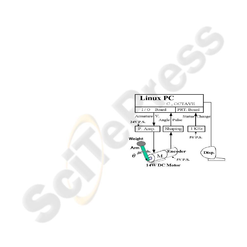
CAD/CAE; Octave and “C” Language (Figure 1).
Using the developed devices, students have flexibly
managed to realise tens of schemes of tangible
theories in the college lab. during last four years.
This paper explains the concepts and
specifications of developed devices, plant modelling
with mathematical linearization. Some developed
applications of modern control theory are introduced.
Finally, three types of discrete–time control methods
for industry uses are applied and their performances
are evaluated in each other.
Figure 1: System configuration.
2 DESIGN CONCEPT AND
SYSTEM CONFIGLATION
The basic component of plant control or Robot can
be reduced to control the position of a arm driven by
a motor. Key points of the design concept and the
spec. of this control system are discussed below.
265
Tanimoto S., Yoshida K. and Tahara J. (2010).
PRACTICAL EDUCATION OF CONTROL ENGINEERING - Using Open OS, Free Software and Actual Plant.
In Proceedings of the 2nd International Conference on Computer Supported Education, pages 265-270
Copyright
c
SciTePress
2.1 Design Concept
2.1.1 Real Time Control
Conventional real time control systems in industries
are controlled every 10 ms. Thanks to the progress
of computer capability today, it is possible to realize
1 ms DDC (Direct Digital Control) by just a P/C.
Once the developed control program is turned on,
the program senses the status change of 1 KHz
oscillator input. this program is executed every 1 ms,
without running OS area at all, achieving the perfect
real-time function.
The sampling time should not be disturbed by
the control calculation time. Because of the 2 GHz
P/C clock, most kinds of optimum calculation are
acceptable for control. Authors did not adopt
commercial real time OS to avoid their complexity
and ambiguity.
2.1.2 Accuracy, Simplicity and Reliability
Actual arm angle can be detected by 14,400 pulses
per rev. through I/O board of the P/C. Control input
to the motor armature is in analogue through 10-bit
DAC. A backlash-less motor without a gear is
adopted. No redundant devices are included.
A simple system configuration directly
corresponds to its reliability and accuracy. These
devices are neatly packed on a single board.
2.1.3 Maintainability
In plant control applications in industries, the
traceable-ness is quite important. Once a software
bug stalled the plant and destroyed the machinery,
the plant cannot be restarted without fixing the bug.
In case of Windows PC, whose source codes are
not disclosed, this bug cannot be fixed. Therefore,
Authors adopted Linux OS of open source code.
2.1.4 Flexible Control Design Capability
Although, AC motors are commonly used instead of
DC motors today, Authors adopted a DC motor for
the arm control, because a DC motor can be easily
expressed by differential equations, which results in
better understanding for users or students.
The controller is designed in C-language and its
PID control reference software is initially installed
by a author. Users can only modify this software for
their own purpose. The input and output of this
controller are the pulse count of the pendulum angle
and the armature voltage of the DC motor,
respectively.
2.1.5 Computer Aided Engineering
This system includes a control CAD/CAE called by
Octave of free software instead of expensive Matlab.
Users can get the chart of controlled result by storing
the control variables in the software table every 1
ms. Octave also offers tools of control theory such
as eigen value, Ricatti solution and transfer function.
Users can compare the actual control results with the
modelled theoretical result by both charts.
2.1.6 Exclusion of Non-linearity in Devises
Authors believe that the mechanical non-linearity
such as backlash, friction and dead time are difficult
to be evaluated and also its fine repeatability is not
realized in actual plants. In the devices here, those
non-linearity are excluded as much as possible. The
gearless motor and the directly coupled encoder with
fine resolution are adopted.
In case of developing those non-linear control
methods, non-linearity should be realized in the P/C
through its software with repeatability. And then,
developed control scheme for pure non-linearity will
be applied to the actual field, and analyzed.
2.1.7 Cost and Open Documents
4 same systems are developed. Its cost is $3,000/set
excluding authors’ labour. This reasonable cost can
mainly be realized by adopting the free software of
Linux and Octave. Its specification is open by
authors to any other groups for education and non-
business use.
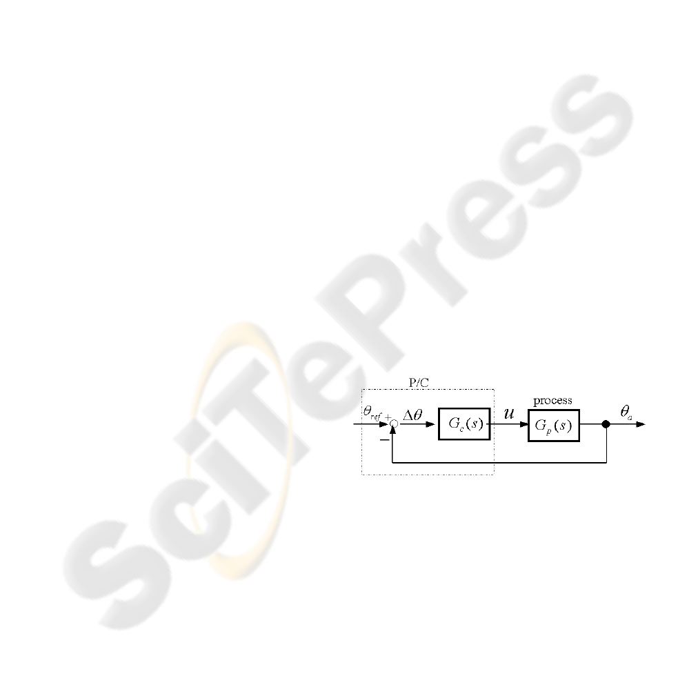
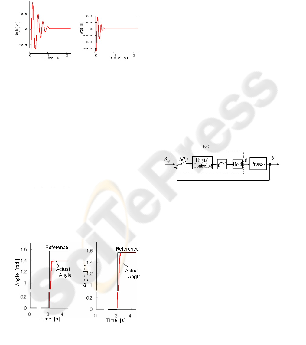
Figure 2: Control Block Diagram.
2.2 Hardware
This system consists of controlled process or plant
and a controller (Figure 2).
2.2.1 Process
a. Motor and Encoder
A small DC motor is adopted considering users’
safety. Rating specifications are on Table 1. Low
inertia-ed rotary encoder directly coupled with the
CSEDU 2010 - 2nd International Conference on Computer Supported Education
266
motor shaft is adopted. Pulse rate is 14,400
pulses/rev.
b. Amplifier and Power Supply
Large capacity-ed power amp. Is adopted
considering the motor stall current (table 2).
Switching power supply for the power amp. Is of
100w with 24vdc and 4.5a.
c. Oscillator
1 KHz oscillator is made as a sampler.
Table 1: Motor spec. Table 2: Amp. spec.
Power
14 W
Power
125 W
Voltage
DC100
Voltage
100 V
Speed
2500 pm
Current
15 A
Torque
0.054 m
2.2.2 Controller
a. P/C
P/C has a CPU of 2 GHz, 256MB memory and
80GB H/D.
b. I/O Board
1 ms sampling signal is input to the printer port .
Analogue i/o; PCI- 3523A has DAC with
12bits, ADC and a few DI/DO.
Encoder counter; PCI-6204 has a 32-bit
counter.
2.3 Software
Linux Fedora Core 1 is adopted for OS. Application
task can access I/O through developed sub-systems
without OS.
Octave for Linux is down loaded. Its application
manual is openly supplied by Internet.
Reference PID control program is prepared. It
has the strict correspondence with its documentation,
block diagram and naming rule. It has blocks of
control parameter initial input, periodical run loop,
data acquisitions, PID calculation, Output to i/o
board and data storing for Octave. Users can modify
this program for their own purposes.
3 PLANT MODELING
Once the plant H/W is designed, then the advanced
control needs its mathematical modelling
3.1 Mathematical Model of the Plant
A motor with a pendulum arm is shown by Figure 3.
Figure 3: DC motor and a pendulum.
These plants are mathematically expressed by
tmglttbtJ
sin
(1)
)(tiKt
T
(2)
)()()()( tKtRitiLtu
V
(3)
Definition of variables and parameters are as follow:
u
: Armature voltage
R
: Armature resistance
L
: Armature inductance
i
: Armature current
b
: Friction loss
J
: Arm inertia
: Motor torque
: Arm angle
l
: Arm length
m
: Mass of Weight
g
: Gravity acc. KT:Torque const.
KV:B.E.F. const.
3.2 Linearization of the Plant
This plant has a non-linear term of
sin
. We need
a linear model to apply the linear control theory. In
conventional method, this term is approximated
by
. Another method adopted here is the strict
linearization by non-linear term compensation.
3.2.1 Approximated Linear Model
Assuming
sin
, 3rd
order model is expressed by
the state variable expression bellow:
u
u
L
i
L
R
L
K
J
K
J
b
J
mgl
i
V
T
bxA
x
1
0
0
0
010
(4)
Incidentally, the inductance L in the DC motor is
ignored in many applications considering the large
amount of the inertia of the arm, which is called 2nd
order model.
PRACTICAL EDUCATION OF CONTROL ENGINEERING - Using Open OS, Free Software and Actual Plant
267
3.2.2 Strictly Linearized 2nd
Order Model
The original system has the serious non-linearity of
t
sin
.
Authors applied the input linearization to
delete non-linearity. (1) can be modified below:
)(sinsin
mglmglbJ
(5)
The term
tt
sin
is compensated to
the motor armature voltage every 1 ms (Figure 4),
getting the linear model as follow:
mglbJ
(6)
By adding this compensation, control theory in
textbooks can be applied without any contradiction.
ref
a
u
Linear
Controller
Motor and
Pendulum
aa
T
K
Rmgl
sin
ref
a
u
Linear
Controller
Motor and
Pendulum
Motor and
Pendulum
aa
T
K
Rmgl
sin
Figure 4: Real time input linearization.
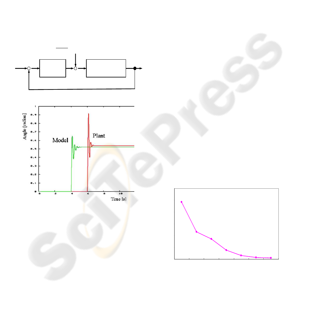
Figure 5: Step response by PID controller.
3.2.3 Identification of the Plant
The derived 2nd
order model is identified to the
actual plant (Figure 5). Both model and actual plant
are controlled by the same PID controller. The
model is executed every 1 ms using Euler difference
method. Incidentally, the dead time of this system is
confirmed to less than 2ms.
4 CONTROL APPLICATIONS
Authors examined several control schemes in text-
books. Basically, control is executed every 1ms,
which is almost regarded as a continuous system.
Every nonlinear function such as dead time,
sampling period, discrete time, saturation, dead zone,
static friction is realized by “C” in P/C. The lists of
developed schemes are as follow:
PID control.
Position control.
Angle velocity control.
Dead time control.
Sampling control.
Control with low resolution sensor.
Control with less number of effective digits.
Modern control with 2nd order.
State feedback control.
Pole assignment control.
Optimum regulator.
Integral type control.
Observer coupled control.
Discretized State feedback control.
Modern control with 3rd order, under work.
Observer coupled control (armature current
observance).
4.1 PID Performance by Sampling
Time
In actual plants, control performance mainly
depends on the sampling period. Continuous
feedback control is desirable.
Authors checked how the control performance
depends on the sampling period quantitatively.
Maximum stable proportional gain Kp for the
horizontal pendulum position control depending on
every sampling period is shown by Figure 6.
0
50
100
150
200
250
300
1 5 10 20 40 80 160
Sampling Period [ms]
Gain Kp
Figure 6: Maximum proportional feedback gain vs.
sampling period.
4.2 Pole Assignment Control
During the state feedback control using 2nd order
CSEDU 2010 - 2nd International Conference on Computer Supported Education
268
plant model, poles are assigned with
4010,205 jjp
using Octave. Control
results are shown in Figure 7. This means the linear
modern control is realized theoretically enough.
205 jp
4010 jp
Figure 7: Pole assigned step responses.
4.3 Integral Type Optimum Regulator
As control theory says the optimum regulator is just
a gain feedback and offset cannot be deleted
depending on the weight matrix Q as follow:
dturu
TT
u
)(min
0
xQx
(7)
To delete this offset, optimum regulator with
integral element is tested. New integral variable is
defined and sate equation is modified as follow:
(8)
u
JR
K
KK
R
b
JJ
mgl
T
VT
0
0
001
0
11
010
x
(9)
Solving the Ricatti equation using Octave,
integral type method is executed getting a satisfied
result. Here, the optimum regulator without integral
variable is compared (Figure 8).
Figure 8: Optimum regulators, right: integral type.
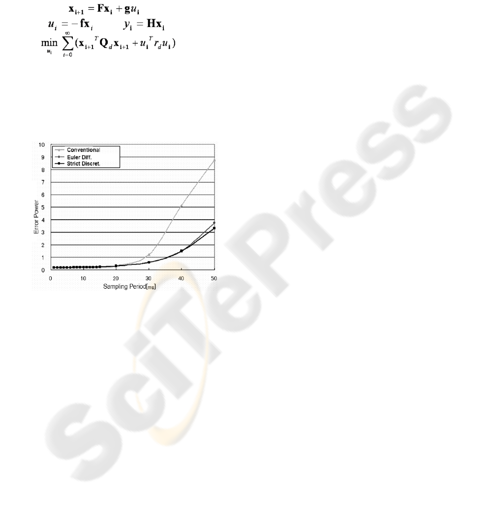
4.4 Discrete Time Control
Performances
4.4.1 Three Kinds of Discretizations
In industry applications, DDC is adopted, where the
sampling time is from a few to 50 ms depending on
the plant dynamics. Figure 9 shows its discrete-time
control block diagram, where T
c
denotes the
calculation time in the sampling period. Authors
checked how the control performance depends on
the sampling period quantitatively in modern
control. Three kinds of discrete-time control
schemes are considered.
4.4.2 Conventional Method
The most common method is just to feedback the
state vector with gain matrix derived from the
continuous type Ricatti Equation as follow:
(10)
Figure 9: Discrete time Control System.
This method is not discrete and may be called by
periodical feedback. This is not optimum any longer,
which doesn’t utilize the information of sampling
period. But this is widely applied in industries
because it doesn’t need the plant discrete model.
4.4.3 Euler Difference Method
Euler Difference Method can easily discretize the
continuous plant model even in a plant controller.
Optimal feedback gain matrix
f
is obtained by
discrete-time Ricatti Equation through Octave.
(11)
4.4.4 Strict Discretization
The strict discretization needs to solve the continues
ubAxx
cxy
ii
u kx
dturu
c
T
c
T
u
)(min
0
xQx
ubAxx
cxy
ii
u kx
dturu
c
T
c
T
u
)(min
0
xQx
TuT
i
bxAIx
i1i
)(
ii
cxy
ii
u fx
)(min
0
ii1i1i
xQx
i
uru
d
T
d
T
u
TuT
i
bxAIx
i1i
)(
ii
cxy
ii
u fx
)(min
0
ii1i1i
xQx
i
uru
d
T
d
T
u
PRACTICAL EDUCATION OF CONTROL ENGINEERING - Using Open OS, Free Software and Actual Plant
269
state variable differential equation :
duee
t
)(
0
)(
b0xtx
t
AAt
(12)
i
A
i
A
1i
bxx udee
T
TT
)(
0
)(
(13)
Discrete-time state variable plant model is
derived:
(14)
Optimum feedback gain matrix
f
is also applied
here using Octave. This method is strict as a
discrete-time modification, but it is pretty difficult to
re-calculate F and g in on-line controller in case of
the product lot change or parameter change of
models in industries
Figure 10: Three performances comparison.
4.4.5 Comparison of Three Performances
Three types of above discrete-time methods have
been designed and executed. The step reference
change was given from horizontal arm angle to the
top dead point. Performances are evaluated by the
angle error power. Each weight matrix Q, r of the
evaluation function of quadratic form in optimum
regulator was chosen to get a good result for 1 ms
sampling period control. And this was fixed during
different sampling period tests.
There may be some discussion about fixing the
evaluation matrix for each to keep the fair
comparison. Basically, the control sampling time
should be related to the plant time constant. In
authors’ plants, velocity response time constant is
0.6 s.
Figure 10 shows the results where different
sampling periods were adopted for these three
methods. These tests gave us the considerable
information that the conventional method resulted in
poor performance especially when the sampling
period is moderately long ,above 20ms. This is why
this method does’t have the information of sampling
period
T
.
On the other hand, authors got relatively good
result by Euler method which is easy to apply
compared to the Strict descretization.
In each discrete time control method, it is
important that the sampling period should be small
under coping over data acquisition and output time
through network.
5 CONCLUSIONS
Authors developed practical educational devices for
students to make them experience the on-line real
time plant control.
Advanced control theories were applied and
those results were checked tangibly. Every trouble
derived from actual plant such as saturation of the
amplifier, cogging of the DC motor, vibration of the
plant, static friction and “C” coding is experienced
by students.
Authors are now working for 3rd order discrete
model with a observer which is giving us delicate
problems of sampling period and pole assignments
of the regulator and observer
Authors confirmed the importance of tangible
control experiment devices for the control
engineering education by the 4 year experience of
sending out about 40 students to industry fields.
REFERENCES
Hanyuda, S. et. al. 2007. Applications of Pendulum
Control System for Developed Educational
Experiment Devices, Risp International Workshop on
Nonlinear Circuits and Signal Processing, Shanghai,
pp.189-192, 2007/3
Tahara, J. et al. 2003. Design of Real Time Controller with
General Linux , Society of Signal Processing
Applications and Technology of Japan, pp 17-21
Vol.6, No.2, 2003/6
CSEDU 2010 - 2nd International Conference on Computer Supported Education
270
