
HANDLING REPEATED SOLUTIONS TO THE PERSPECTIVE
THREE-POINT POSE PROBLEM
Michael Q. Rieck
Drake University, U.S.A.
Keywords:
P3P, Pose, Photogrammetry, Danger cylinder, Discriminant, Jacobian, Repeated solution, Double solution.
Abstract:
In the Perspective 3-Point Pose Problem (P3P), when the three reference points are equidistant from each
other, this distance may be assumed to be one unit in length. A repeated solution to the problem then occurs
when and only when 1 + R
1
R
2
+ R
2
R
3
+ R
3
R
1
−R
2
1
−R
2
2
−R
2
3
= 0, where R
1
,R
2
and R
3
are the squared
distances from the camera’s focal point to the reference points. When the setup only approximately satisfies
this equation, two nearly equal solutions can introduce substantial calculation errors. To better handle this
circumstance, it may be preferable to behave as though the above equation holds precisely, and then invert
a certain two-dimensional transformation to obtain the repeated solution. The inversion involves only a few
basic arithmetic operations and square roots. This approach is more efficient, and more reliable, than the
standard quartic equation approach to solving P3P, at least in this special case.
1 INTRODUCTION
The Perspective 3-Point Pose Problem (P3P), as in-
troduced and solved by J. A. Grunert (1841), is essen-
tially concerned with inferring the distances to three
known reference points, seen in a photograph, from
the camera that took the photograph. With this in-
formation, one can then determine the position and
orientation of the camera. Amazingly, the problem is
nearly as old as photography itself.
Traditionally its applications were restricted to ar-
eas of photogrammetry such as aerial reconnaissance.
More recently though, it has been successfully ap-
plied in electronic digital imaging to address a vari-
ety of practical problems. These include robotic con-
trol and navigation, as in (Qingxuan, et al, 2006),
as well as six-degree-of-freedom tracking for vir-
tual/augmented reality and video game applications,
as in (Chen, et al, 1998) and (Ohayon and Rivlin,
2006).
Advancements and refinements in the study of
P3P were steadily made throughout the nineteenth
and twentieth century, as for example (Merritt, 1949)
and (M
¨
uller, 1925). An extensive survey of the state
of P3P as of 1994 can be found in (Haralick, et al,
1994). Several recent studies have classified solu-
tions, such as (Faug
`
ere, et al, 2008), (Gao, et al,
2003), (Wolfe, et al, 1991), (Zhang and Hu, 2005)
and (Zhang and Hu, 2006).
A simplified version of P3P assumes that the dis-
tances between the three reference points are equal.
Attention will be limited in the following discussion
to this situation, where in fact, the measurement units
will be set so as to make this distance equal one. The
P3P problem assumes that the cosines of the inte-
rior angles between pairs of lines-of-sight to the refer-
ence points are known, and that one wishes to deter-
mine the distances to these points. These cosines are
straightforward to calculate from the photograph (or
digital image) and intrinsic camera properties. Us-
ing the Law of Cosines, the underlying mathemati-
cal problem to be solved is therefore the determina-
tion of the unknown values of r
1
,r
2
,r
3
, based on the
known values of c
1
,c
2
,c
3
, in the following system of
quadratic equations:
r
2
1
+ r
2
2
−2c
3
r
1
r
2
= 1
r
2
2
+ r
2
3
−2c
1
r
2
r
3
= 1
r
2
1
+ r
2
2
−2c
2
r
3
r
1
= 1.
(1)
It will be convenient to set R
j
= r
2
j
( j = 1,2, 3),
and to sometimes regard (1) as a system of equations
in R
1
,R
2
and R
3
. As demonstrated by Grunert, it is
possible to eliminate any two of the three unknowns,
resulting in a single quartic (i.e. fourth degree) poly-
nomial equation in the remaining R
j
(for j = 1,2,3):
AR
4
j
+ B
j
R
3
j
+C
j
R
2
j
+ D
j
R
j
+ E
j
= 0. (2)
395
Q. Rieck M. (2010).
HANDLING REPEATED SOLUTIONS TO THE PERSPECTIVE THREE-POINT POSE PROBLEM.
In Proceedings of the International Conference on Computer Vision Theory and Applications, pages 395-399
DOI: 10.5220/0002790103950399
Copyright
c
SciTePress

The coefficients here depend on c
1
,c
2
and c
3
. The
leading coefficient A, as well as the equation’s dis-
criminant ∆, turn out (surprisingly) to be independent
of j. Specifically, A = 16 T
2
and
∆ = 16777216 (c
2
1
−c
2
2
)
2
(c
2
2
−c
2
3
)
2
(c
2
3
−c
2
1
)
2
T
2
S,
(3)
where
T = 1 + 2τ −σ , S = (4)
4(1 −τ)
2
(1 + 8τ) T − 3 [ 3χ −(1 + 2τ)
2
]
2
,
σ = c
2
1
+c
2
2
+c
2
3
, τ = c
1
c
2
c
3
, χ = c
2
1
c
2
2
+c
2
2
c
2
3
+c
2
3
c
2
1
.
The computations involved here are rather tedious,
and best checked using mathematical manipulation
software, such as Mathematica
R
or Maple
TM
.
1
The
polynomial S appears to be irreducible. However, the
story changes when the c
j
are expressed in terms of
the r
j
, using the following rational transformation:
c
1
=
r
2
2
+ r
2
3
−1
2r
2
r
3
, c
2
=
r
2
3
+ r
2
1
−1
2r
3
r
1
, c
3
=
r
2
1
+ r
2
2
−1
2r
1
r
2
,
(5)
obtained by solving (1) for the c
j
(when the r
j
are all
nonzero). This transformation causes S to factor as
S = Ω
2
H / 256 R
4
1
R
4
2
R
4
3
, (6)
where
Ω = 1 + R
1
R
2
+ R
2
R
3
+ R
3
R
1
−R
2
1
−R
2
2
−R
2
3
, (7)
and where H is a rather complicated eighth degree
polynomial in R
1
,R
2
and R
3
. Moreover, the Jacobian
determinant of the transformation (5) is
J = Ω/4r
3
1
r
3
2
r
3
3
. (8)
Section 2 describes the singular situation that re-
sults when two solutions coalesce to form a double
solution, causing J to vanish. This is “singular” in
the sense that transformation (5) from (r
1
,r
2
,r
3
) to
(c
1
,c
2
,c
3
) becomes locally non-invertible.
The principal result of this article is next pre-
sented, an efficient algorithm called as “DSA” for
handling double solutions. Section 2 also discusses
the results of experiments conducted using this algo-
rithm. Section 3 studies the transformation (5), from
the r
j
to the c
j
, in more detail, and lays the mathemat-
ical foundation for DSA.
1
A Mathematica notebook is available upon request.
2 DOUBLE SOLUTIONS
2.1 Double Solutions as Error Sources
This article is concerned with the situations where
Ω = 0 (hence J = S = ∆ = 0), and where |Ω| is suffi-
ciently close to zero to cause trouble. Since J tends to
be small when |Ω| is small, computational errors can
result in large errors when computing the values of the
r
j
from those of the c
j
. This situation occurs when
two solutions to the quadratic system (1) coalesce
or nearly coalesce into a double solution. The case
where Ω = 0 was introduced and studied in (Smith,
1965) and (Thompson, 1966), and later considered by
others, such as (Zhang and Hu, 2005) and (Zhang and
Hu, 2006). It turns out that Ω = 0 corresponds to hav-
ing a physical setup in which the camera’s focal point
is on a special circular cylinder, customarily known as
the “danger cylinder.”
When S = 0, it can be shown that Ω = 0 for some
solution to (1), which is thus a repeated solution. By
determining that |S| is smaller than some given toler-
ance, and then behaving as though S = 0, the (nearly)
repeated solution can be computed more efficiently
and reliably than would otherwise be the case. Rather
than solving Grunert’s complicated quartic polyno-
mial, or following any of several known equivalent
approaches, one only needs to follow a simple algo-
rithm, detailed in the next subsection. As will be seen,
this only requires a few basic computations, involving
nothing more complicated than square roots.
There are a couple reasons why behaving as
though S = 0, when |S| is small, might be prudent.
Imprecisions in measuring the c
j
and/or roundoff er-
ror in computing S, mean that it might be impossible
to know for certain if S is zero, positive, negative, or
even non-real. Since the discriminant of the quartic
polynomials involves S as a factor, it is possible that
two nearly equal real solutions (or a double solution)
are erroneously perceived to be complex solutions in-
stead, and thereby ignored as being physically unre-
alistic. Even when two nearly equal real solutions are
discovered, these are likely to be rather far from the
correct solutions, owing to the small value of the Ja-
cobian determinant.
2.2 Double Solutions Algorithm (DSA)
The following algorithm has been found to be a sim-
ple way to mitigate the difficulties caused by double
solutions:
1. Receive (c
1
,c
2
,c
3
) as input.
2. If necessary, negate any two of c
1
,c
2
and c
3
, so
as to make c
1
+ c
2
+ c
3
≥
1
2
. If this is not possi-
VISAPP 2010 - International Conference on Computer Vision Theory and Applications
396

ble, then quit, indicating that there is no repeated
solution.
3. Compute σ,τ,χ, T and S, using formulas (4).
4. If |S| is sufficiently small, then behave as though
S = 0, and continue this algorithm; otherwise quit,
indicating that there is no repeated solution.
5. Solve for u and v, using formulas (13). These for-
mulas uniquely determine a u with u ≥ 0, and a v
with |v| ≤ 1 (as can be proved).
6. Compute tentative values for r
1
,r
2
and r
3
using
formulas (10), and r
j
=
p
R
j
( j = 1,2,3).
7. Compute corresponding values for c
2
and c
3
using
formulas (5). Call these c
0
2
and c
0
3
though.
8. Test to see whether or not swapping c
0
2
and c
0
3
would cause them to be closer to the values of c
2
and c
3
(from step 2). If so, then swap r
2
and r
3
.
9. If any negation took place in step 2, then com-
pensate for this by now negating a corresponding
r
1
,r
2
or r
3
. Negate r
1
if c
2
and c
3
were negated;
negate r
2
if c
1
and c
3
were negated; negate r
3
if c
1
and c
2
were negated.
10. Return the repeated solution (r
1
,r
2
,r
3
).
Note that system (1) (using altered or unaltered c
j
)
has a repeated solution if and only if S = 0, and except
in some very special cases, a repeated solution is only
a double solution. Also, “closeness” in step 8 might
be decided by considering (c
0
2
−c
2
)
2
+(c
0
3
−c
3
)
2
ver-
sus (c
0
2
−c
3
)
2
+ (c
0
3
−c
2
)
2
. Although the correctness
of this algorithm is not proven here, the mathematical
analysis that led to it is described in Section 3. Addi-
tionally, the simulations to be discussed next attest to
its correctness as well.
2.3 Simulations
Simulations confirm the advantages of using the Dou-
ble Solution Algorithm when |S| is small. These sim-
ulations were performed using compiled Mathemat-
ica functions, running on an Intel Core Duo processor.
Thus the floating point computations were performed
using 64-bit IEEE floating point format. Even more
dramatic results can be expected in a 32-bit floating
point environment.
A radius-one danger cylinder was used. Five dif-
ferent distance ranges along the cylinder axes were
explored: 0-2, 2-4, 4-6, 6-8 and 8-10. A camera focal
point on the cylinder (within the given range) was ran-
domly selected, and the cosines c
1
,c
2
,c
3
computed.
DSA was tested against Grunert’s quartic polynomial
method, and the resulting computed distances for r
1
were compared with the actual value of r
1
.
Next, each of the three cosines was randomly
perturbed by adding or subtracting up to one one-
millionth to/from it, and the two methods were com-
pared again using the resulting data. This was again
repeated, but using a maximum adjustment of one
one-hundredth, rather than one one-millionth, for
each cosine. In this way, fifteen different experi-
ments (five distance ranges times three maximum co-
sine perturbation amounts) were considered. Each of
these experiments was performed one hundred thou-
sand times, and the results of these trials were aver-
aged.
When the computed cosines (c
1
,c
2
,c
3
) for a point
(essentially) on the danger cylinder were left unper-
turbed, the ratio of the average errors using Grunert’s
method versus DSA was between a hundred million
and a billion. Admittedly though, the likelihood of
having the camera’s focal point right on the danger
cylinder, within the computational tolerance of 64-
bit floating point arithmetic, is very small. Thus fur-
ther experiments were conducted using slightly al-
tered value of the cosines.
When the cosines were randomly perturbed by an
amount up to one one-millionth, the ratio of the av-
erage computed errors was as much as 52, when the
focal point was close to the reference point (the 0-2
range). But this ratio dropped to 14 when the focal
point was far away (8-10 range).
When the cosines were randomly perturbed by
an amount up to one one-hundredth, the error ratio
ranged between one and two. Thus the improvement
using DSA was modest in this case. Once again
though, computations performed using 32-bit arith-
metic, instead of 64-bit arithmetic, would more dra-
matically demonstrate a difference in accuracy be-
tween the two methods.
The ratio of the execution times for the two meth-
ods were also compared. Here though, it was difficult
to know how much of the timing reported by Math-
ematica was attributable to the overhead involved in
calling compiled functions from within the Mathe-
matica interpreter. In every case, the reported speedup
(ratio) was in excess of four. However, a quick check
of the actual computations involved in the two meth-
ods suggests that the true speedup should be consid-
erably higher.
3 MATHEMATICAL ANALYSIS
This section captures much of the reasoning underly-
ing DSA. The phrases “R-space,” “r-space” and “c-
space” will be used to refer to the abstract three-
dimensional spaces of (R
1
,R
2
,R
3
) points, (r
1
,r
2
,r
3
)
HANDLING REPEATED SOLUTIONS TO THE PERSPECTIVE THREE-POINT POSE PROBLEM
397
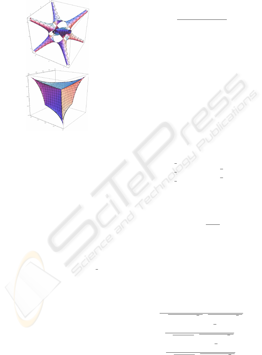
Figure 1: The critical surfaces
b
Q and
b
S.
points, and (c
1
,c
2
,c
3
) points, respectively. Because
the coordinates of the points in c-space represent the
cosines of angles in physical space, we are particu-
larly interested in the points (c
1
,c
2
,c
3
) whose coordi-
nates have absolute value less than or equal to one.
Let
b
T denote the set of points in c-space for which
|c
j
| ≤ 1 ( j = 1, 2,3) and T ≥ 0 (another physical
requirement). The boundary of this region (where
T = 0) is shaped like an “inflated tetrahedron,” basi-
cally resembling an over-stuffed tetrahedral pillow.
b
T
consists of this surface plus its interior. Let
b
S denote
the set of all points in
b
T satisfy the equation S = 0.
This surface is shown on the right in Figure 1. It re-
sembles a deformed cube with two types of vertices,
all of which are also on the boundary of
b
T .
b
S can
be decomposed into four identical sections, each re-
sembling a deformed triangular cone. One of these
consists of points satisfying c
1
+c
2
+c
3
≥
1
2
, referred
to as the “principal cone.”
In r-space, there are also restrictions on the set of
points (r
1
,r
2
,r
3
) that are realizable, given the setup in
physical space. Since the reference points are a dis-
tance one apart, it is immediately clear that no two of
r
1
,r
2
and r
3
can differ by more than one. There is
an additional restriction though, imposed by the fact
that the tetrahedron, in physical space, whose vertices
are the camera’s focal point and the three reference
points, must have positive volume. Using the Cayley-
Menger determinant, it can be seen that 144 times this
volume equals Ω + R
1
+R
2
+R
3
−2. So it is required
that this be non-negative. Also, a quick check estab-
lishes that when the substitution (5) is used to express
T in terms of the r
j
, one obtains
T =
Ω + R
1
+ R
2
+ R
3
−2
4R
1
R
2
R
3
. (9)
Let
b
R denote the region in r-space consisting of
points (r
1
,r
2
,r
3
) satisfying |r
1
−r
2
| ≤ 1, |r
2
−r
3
| ≤
1, |r
3
−r
1
| ≤ 1 and Ω + R
1
+ R
2
+ R
3
≥ 2. These are
the points in r-space that are physically realizable, as-
suming that negative values of r
j
are admissible.
Let
b
Q denote the subset of
b
R consisting of points
for which Ω = 0. This surface is shown on the left in
Figure 1. Because of (6), it is clear that the points of
b
Q (in r-space) correspond to points of
b
S (in c-space),
under the transformation (5). It can be shown that
this mapping from
b
Q to
b
S is onto, except for a set of
measure zero.
From equation (7), observe that the surface
b
Q cor-
responds to a portion of a circular cylinder in R-space.
Only a portion of the cylinder is admissible though,
due to the restriction that R
1
+ R
2
+ R
3
≥ 2, by (9),
since T ≥ 0 and Ω = 0. The semi-cylinder (surface)
can be parameterized as follows:
R
1
=
1
3
(2 + u −2 cos θ),
R
2
=
1
3
(2 + u + cos θ +
√
3sin θ),
R
3
=
1
3
(2 + u + cos θ −
√
3sin θ).
(10)
Here u = R
1
+ R
2
+ R
3
− 2, which must be non-
negative, and we will assume too that 0 ≤ θ < 2π.
Notice that replacing θ with θ ±2π/3 (mod 2π) in-
duces a cyclic permutation of {R
1
,R
2
,R
3
}. Replacing
θ with 2π −θ swaps R
2
and R
3
. It is helpful to use the
notation v = cosθ and w = ±
√
1 −v
2
= sin θ.
Because of the independent sign choices for each
of r
1
,r
2
and r
3
, for given R
1
,R
2
and R
3
, there are eight
identical sections, or “legs,” of
b
Q in r-space. These
correspond to the same semi-cylinder in R-space, with
u ≥ 0. The section for which r
1
,r
2
and r
3
are all non-
negative will be called the “principal leg” of
b
Q . The
points on the principal leg of
b
Q get mapped, via (5),
to points on the principal cone of
b
S. Expressing points
on the principal leg in terms of u,v and w, the mapping
(5) becomes the following:
c
1
=
1 + 2u + 2v
2
p
2 + u + v +
√
3w
p
2 + u + v −
√
3w
,
c
2
=
1 + 2u −v −
√
3w
2
√
2 + u −2v
p
2 + u + v −
√
3w
,
c
3
=
1 + 2u −v +
√
3w
2
√
2 + u −2v
p
2 + u + v +
√
3w
.
(11)
VISAPP 2010 - International Conference on Computer Vision Theory and Applications
398

These formulas then lead immediately to the follow-
ing formulas:
σ =
6(1 + 3v −4v
3
) + 3u(3 + 12u + 4u
2
)
4(2 + u −2v)(1 + 4u + u
2
+ 4v + 4v
2
+ 2uv)
,
τ =
(1 + 2u + 2v)(−1 + 2u + 2u
2
−v + 2v
2
−2uv)
4(2 + u −2v)(1 + 4u + u
2
+ 4v + 4v
2
+ 2uv)
,
χ =
3(1 + 3v −4v
3
)
2
+
3u(1 + 3v −4v
3
)(3 + 3u + 4u
2
)
+ 6u
3
(3 + u)(3 + 6u + 2u
2
)
4(1 + 4u + u
2
+ 4v + 4v
2
+ 2uv)
2
.
(12)
As complicated as formulas (11) and (12) are,
surprisingly simple inversion formulas exist. Given,
c
1
,c
2
and c
3
, and using (4) to compute σ and τ, the
values of u and v can be readily deduced from the fol-
lowing:
(1 + u)
2
=
3(1 + 8τ)
4(1 + 2τ −σ)
,
(1 + v)
2
=
3(1 + 2τ −3c
2
2
)(1 + 2τ −3c
2
3
)
4(1 + 2τ −3c
2
1
)(1 + 2τ −σ)
. (13)
These two formulas can be efficiently confirmed us-
ing mathematical manipulation software, by making
substitutions using (11) and (12).
4 CONCLUSIONS
The Double Solution Algorithm (DSA) presented in
this article gives a very practical, very fast, and highly
accurate method for solving the P3P problem, when
dealing with the setup where the camera’s focal point
is on or near the danger cylinder, and when the ref-
erence points are equidistant from each other. It re-
lies on the inversion of a transformation between two
surfaces. Surprisingly, the inverse mapping turns out
to be simpler to compute than the original mapping.
It would be quite useful to find a generalization of
DSA to the situation where the reference points are
no longer assumed to be equidistant from each other.
REFERENCES
Chen C-S, Hung Y-P, Shih S-W, Hsieh C-C, Tang C-Y,
Yu C-G and Chang Y-C (1998). Integrating virtual
objects into real images for augmented reality. In
VRST’98, ACM Symp. Virtual Reality Software and
Techology, pp. 1-8. ACM.
Faug
`
ere J-C, Moroz G, Roullier F, El Din M S (2008).
Classification of the perspective-three-point problem,
discriminant variety and real solving polynomial sys-
tems of inequalities. In ISSAC’08, 21st ACM Int.
Symp. Symbolic and Algebraic Computation, pp. 79-
86. ACM.
Gao X-S, Hou X-R, Tang J, and Cheng H-F (2003). Com-
plete solution classification for the perspective-three-
point problem. In IEEE Trans. Pattern Analysis and
Machine Intelligence, v. 25, n. 8, pp. 930-943. IEEE.
Grunert J A (1841). Das pothenotische problem in er-
weiterter gestalt nebst
¨
uber seine anwendungen in der
geod
¨
asie. In Grunerts Archiv f
¨
ur Mathematik und
Physik, Band 1, pp. 238-248. Verlag von C. A. Koch.
Haralick R M, Lee C-N, Ottenberg K and N
¨
olle N (1994).
Review and analysis of solutions of the three point
perspective pose estimation Problem. In J. Computer
Vision, v. 13, n. 3, pp. 331-356. Springer Netherlands.
Merritt, E L (1949). Explicit three-point resection in space.
In Photogrammetric Engineering, v. 15, n. 4, pp. 649-
655. Amer. Soc. Photogrammetry.
M
¨
uller F J (1925). Direkte (exakte) l
¨
osung des einfachen
r
¨
uckw
¨
artsein-schneidens im raume. In Allegemaine
Vermessungs-Nachrichten. Wichmann Verlag.
Ohayon S and Rivlin E (2006). Robust 3D head tracking
using camera pose estimation. In ICIP’06, Int. Conf.
Image Processing, pp. 1063-1066. IEEE.
Qingxuan J, Ping Z and Hanxu S (2006). The study of po-
sitioning with high-precision by single camera based
on P3P algorithm. In INDIN’06, IEEE Int. Conf. In-
dustrial Informatics, pp. 1385-1388. IEEE.
Smith A D N (1965). The explicit solution of the single
picture resolution problem, with a least squares ad-
justment to redundant control. In Photogrammetric
Record, v. 5, n. 26, pp. 113-122. Wiley-Blackwell.
Thompson E H (1966). Space resection: failure cases. In
Photogrammetric Record, v. 5, n. 27, pp. 201-204.
Wiley-Blackwell.
Wolfe W J, Mathis D, Sklair C W, and Magee M (1991).
The perspecive view of three points In IEEE Trans.
Pattern Analysis and Machine Intelligence, v. 13, n. 1,
pp. 66-73. IEEE.
Zhang C-X and Hu Z-Y (2005). A general sufficient condi-
tion of four positive solutions of the P3P problem. In
J. Comput. Sci. & Technol., v. 20, n. 6, pp. 836-842.
Springer.
Zhang C-X and Hu Z-Y (2006). Why is the danger cylinder
dangerous in the P3P problem? In Acta Automatica
Sinica, v. 32, n. 4, pp. 504-511. Elsevier.
HANDLING REPEATED SOLUTIONS TO THE PERSPECTIVE THREE-POINT POSE PROBLEM
399
