
REAL-TIME ROAD SCENE CLASSIFICATION USING INFRARED
IMAGES
David Forslund, Per Cronvall and Jacob Roll
Autoliv Electronics AB, Linköping, Sweden
Keywords:
Scene classification, Bag of words, Visual words.
Abstract:
This paper aims at employing scene classification in real-time to the two-class problem of separating city and
rural scenes in images constructed from an infrared sensor that is mounted at the front of a vehicle. The ’Bag
of Words’ algorithm for image representation has been evaluated and compared to two low-level methods
’Edge Direction Histograms’, and ’Invariant Moments’. A method for fast scene classification using the Bag
of Words algorithm is proposed using a grey patch based algorithm for image element representation and a
modified floating search for visual word selection. It is also shown empirically that floating search for visual
word selection outperforms the currently popular k-means clustering for small vocabulary sizes.
1 INTRODUCTION
In image processing, scene classification is a fun-
damental task. Providing semantic labels to image
scenes is beneficial as a preparatory step for further
processing, such as object recognition. In the applica-
tion of intelligent vehicles a real-time scene classifica-
tion can be useful both during day and night time. For
the night time case a visual camera cannot be used and
an alternative imaging device, e.g. an infrared sensor,
is required. This paper applies the task of scene clas-
sification to the field of real-time infrared vision sys-
tems, but the proposed methods generalise well also
to grey-scale images. Emphasis is laid on proposing a
system suitable for the real-time two class application
of separating city and rural road scenes. There are
two major sides to scene classification: image repre-
sentation and classification. For image representation,
the Bag of Words (BoW) framework, which describes
the image through the distribution of small image el-
ements, visual words, has been employed and com-
pared to two low-level image representation methods,
Edge Direction Histograms (EDH) and Invariant Mo-
ments (IM). For classification we used two classifiers:
Support Vector Machines (SVM) using radial basis
kernels as implemented in (Chang and Lin, 2001), and
k-Nearest Neighbour (kNN). Due to a larger mem-
ory demand, kNN in its original formulation is not
suited to be used for the real-time system, but is re-
garded as a reference for evaluation purposes. In the
BoW framework k-means clustering is traditionally
used for the formation of the visual vocabulary. This
paper uses a modified version of the floating search
algorithm initialised by k-means for this task, which
gives a vocabulary adapted to the specific classifica-
tion task at hand. Our contributions are firstly, treat-
ment of scene classification in infrared images, and
secondly, emphasis on solving the real-time problem.
Contributions to the BoW algorithm are investigation
of the use of very small vocabularies and the use of
floating search for visual vocabulary construction.
2 RELATED WORK
Scene classification is a mature field in image pro-
cessing, and a variety of approaches to the task have
been investigated. However, few of these deal with
computationally constrained problems such as real-
time applications. Low-level methods are compu-
tationally cheap and are interesting in this context.
(Vailaya et al., 1998) uses a variety of global low-level
features based on colour histograms, frequency do-
main DCT coefficients and edges, applied to the two
class problem of separating city and landscape im-
ages. Edge based features showed best results. Their
work was extended to involve more than two classes
in (Vailaya et al., 2001). (Oliva and Torralba, 2003)
and (Oliva and Torralba, 2001) utilised the frequency
domain further by studying the statistical properties
of the Fourier spectra of image categories and apply-
ing PCA on the spectra to obtain a feature represen-
351
Forslund D., Cronvall P. and Roll J. (2010).
REAL-TIME ROAD SCENE CLASSIFICATION USING INFRARED IMAGES.
In Proceedings of the International Conference on Computer Vision Theory and Applications, pages 351-356
DOI: 10.5220/0002821503510356
Copyright
c
SciTePress
tation. (Szummer and Picard, 1998) considers tex-
ture features (MSAR) for the indoor-outdoor problem
and compares them to colour histograms and DCT.
They also conclude that performance can be gained
by combining features of different types. Another
low-level approach, invariant moments, were applied
in (Devendran et al., 2007) to the two class prob-
lem of street-highway. The BoW image representa-
tion, which implies an additional abstraction level,
has been applied to the scene classification task with
great success. In particular, it has shown to work well
when there are many classes to categorise. (Quelhas
et al., 2005) studied the three class problem of sep-
arating indoor, city and landscape scenes by apply-
ing a BoW representation using sparse SIFT descrip-
tors and applying probabilistic latent semantic analy-
sis (pLSA) to give a compact representation. Results
were compared to those of the low-level methods de-
fined in (Vailaya et al., 1998), where BoW showed
to be superior. (Bosch et al., 2008) solves a multi-
class problem (13 scenes) also using the BoW algo-
rithm and pLSA. Several image element representa-
tions were evaluated: grey patches, colour patches,
dense grey SIFT, dense colour SIFT and sparse grey
SIFT. The dense SIFT was found to give best per-
formance. A promising recent approach to the BoW
framework is the Bag of Textons (Walker and Malik,
2003) which has been applied successfully to several
complex scene classification problems, e.g. (Battiato
et al., 2008). Textons are however left outside the
scope of this paper. A thorough review of previous
work in scene classification was carried out in (Bosch
et al., 2007).
3 IMAGE REPRESENTATION
The city-rural classes can be assumed to have large
intra-class variability. This allows employing less
complex algorithms while still achievinggood results.
3.1 Bag of Words
BoW originates from text retrieval, but has also been
successfully applied to image processing (Sivic and
Zisserman, 2003). The method involves extracting
local patches, image elements, from each image rep-
resenting them by some descriptor. These are then
quantised by a set of representative descriptors, a vi-
sual vocabulary, where each member is called a vi-
sual word. Each image is represented by a feature
vector, constituted by the occurrence frequencies of
the V visual words. These are measured by matching
extracted image elements to the visual words by Eu-
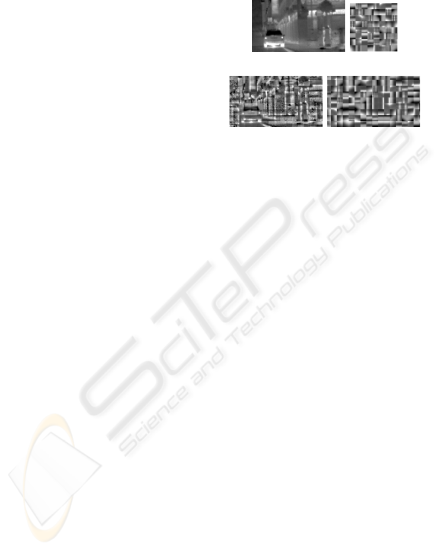
(a) (b)
(c) (d)
Figure 1: An example image (a) is processed (c) by DC
level and std compensated (as in GP-DC). This is compared
to the vocabulary quantisation (d) of (a) by (b) a GP-DC
vocabulary (V=64).
clidian nearest neighbour. Each element of the feature
vector is normalised to range [0 1] on the set of train-
ing images to remove bias towards common words.
Normalisation coefficients are stored in a vector re-
ferred to as the scaling vector. BoW is employed in
this paper, while the lately popular pLSA is not, since
it has shown to give little effect when the number of
scene classes is small (Bosch et al., 2008).
3.1.1 Representation of Image Elements
Image elements can be extracted densely by sampling
across the whole image with a fixed spatial interval or
sparsely by applying an interest point detector. Since
many image elements are extracted from each image,
a simple representation algorithm is desired. The high
abstraction level of the BoW algorithm allows even
such simple representations to result in powerful clas-
sifiers. A basic grey patch descriptor is obtained by
densely sampling square image regions of size n× n
and spacing m giving a descriptor length of n
2
with
a strong bias to visual words describing pure grey-
levels. We denote it GP-Raw. To represent more dis-
criminative structures in the image than grey levels
we remove the DC component from each patch and
normalise the result to std 1. Adding the DC-level as
an extra descriptor gives a descriptor of length n
2
+ 1
which we denote GP-DC. Quantisation of an image
using a vocabulary constructed by the GP-DC repre-
sentation is shown in Figure 1.
To further remove low dimensional structure we
developed two general methods to remove the gradi-
ent component from a patch. In the GP-PL, the patch
is seen as a surface z = f(x, y) where the z is the pixel
intensity. The mean gradient of the patch is removed
by subtracting a plane a z
a
= ax+ by+ c acquired by
least square approximation of z. The result is then
VISAPP 2010 - International Conference on Computer Vision Theory and Applications
352
normalised to std 1 and gradient information is kept
by adding coefficients a, b and c to the descriptor vec-
tor giving length n
2
+ 3. Another way to remove lin-
ear order structures is to remap the grey-levels based
on the histogram of the patch. The cumulative his-
togram q of an image is a monotonically increasing
function, thus the slope d of a least-squares linear ap-
proximation eq is positive with magnitude depending
on the dynamic range of the image. We discretise eq
in terms of the histogram bins and subtract it from
the patch pixels. The result is normalised to std 1.
The patch DC level and the slope d are added to the
descriptor denoted GP-HGM giving it length n
2
+ 2.
Alternatively eq can be discretised for each individual
pixel. To avoid non-deterministicresults, this requires
that the pixels are sorted in a controlled manner within
each histogram grey-level, taking the pixels spatial lo-
cation in the patch into account. We denote this GP-
PS. Figure 2 shows the five GP based descriptors in-
troduced in this section applied to an image patch.
Sparse extraction has been employed using the
DoG detector and the SIFT descriptor as in (Lowe,
2004). The SIFT descriptor has also been applied
densely as in (Bosch et al., 2008). For each sampled
point, SIFT descriptors were then calculated on four
different scales, using circular support patches of radii
4, 8, 12 and 16 pixels.
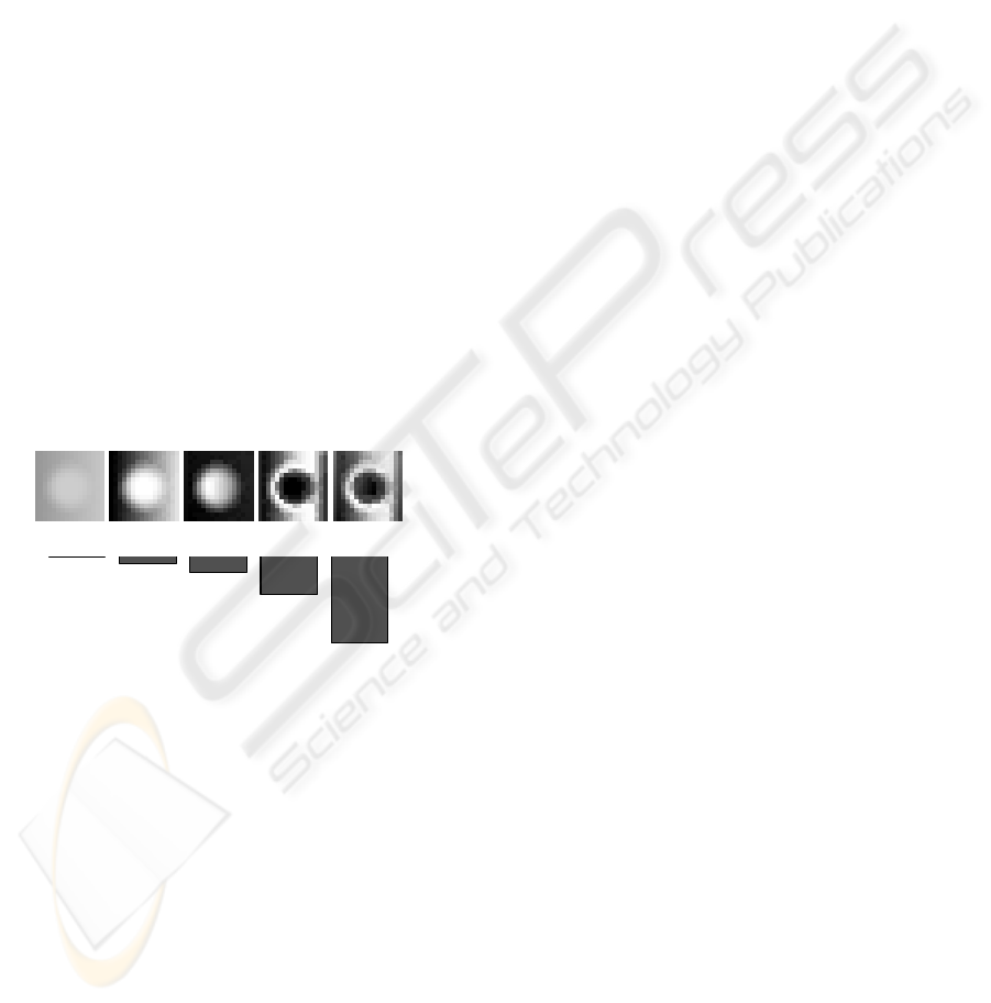
(a) (b) (c) (d) (e)
(f)
Figure 2: An image patch as represented by descriptors: (a)
GP-Raw, (b) GP-DC, (c) GP-PL, (d) GP-HGM, (e) GP-PS.
(f) shows relative time consumption of above descriptors.
3.1.2 Constructing a Visual Vocabulary
The vocabulary should be representative, approximat-
ing all possible image elements occurring in a sam-
ple image, and provide a representation that facilitates
separating the scene classes. To construct a vocabu-
lary, image elements are extracted from a subset of
the image dataset. From these (typically about 1 mil-
lion elements), a small set of a fixed size is created to
constitute the vocabulary. In literature, this has been
carried out by applying k-means clustering to the ex-
tracted image elements, defining the visual words as
the cluster midpoints. This strategy discards informa-
tion of the class membership of the image elements.
We wish to exploit this information to optimise the
vocabulary to the classification task. Thus we employ
floating search (Pudil et al., 1994), which is a feature
selection algorithm designed to select the best subset
of a predefined size out of large set of features. The
subset quality is estimated based on some criterion
function. For the application of this paper, the only
sensible criterion function is the final classification
rate. To obtain an algorithm of manageable speed,
classification is carried out on a subset of 200 images,
and the criterion function is the mean value of a 4-
fold cross validation. To further increase speed, the
floating search algorithm is not allowed to pick from
all reference image elements, but from a set of 400
elements, obtained by k-means clustering the com-
plete set. Since words are matched by nearest neigh-
bour it is impossible to have a vocabulary of only one
word. Thus floating search needs to be initialised with
a two-word vocabulary, which can be found by ex-
haustive evaluation among the 400 candidates, or by
using some fitness measure on the individual image
elements.
3.2 Low-Level Algorithms
Low-Level features are fast to compute and, given
the problem complexity, might provide sufficient per-
formance. Edge direction histograms has shown
(Vailaya et al., 1998) to be efficient for simpler scene
classification tasks. They are well suited for the
city-rural problem, since they exploit the fact that
city scenes contain more vertical structures than ru-
ral scenes. EDH was implemented using both Canny
and Sobel edges, and adding the fraction of non-edge
pixels as an additional feature.
A set of seven central geometric image moments
proposed in (Hu, 1962), that in the discrete 2D case
can be shown to be translation, scaling and rotation
invariant, have been successfully used as features in
many image processing tasks, including scene clas-
sification (Devendran et al., 2007). These were im-
plemented as features by subdividing each image into
four regions and calculating Hu’s seven moments for
each region, giving a feature vector of length 28, nor-
malised by scaling the logarithm of each moment to
the range [0,1] over all training images.
4 TIME AND MEMORY
For a real-time system, time and memory consump-
tion is crucial. The system consists of two stages: the
off-line stage of vocabulary construction and classi-
fier training, which is not severely restricted in com-
REAL-TIME ROAD SCENE CLASSIFICATION USING INFRARED IMAGES
353
putational time, and the on-line stage of feature ex-
traction and classification which needs to be per-
formed at real-time speed. In the experiments clas-
sification time is consistently seen to be negligible
in comparison to feature extraction, which here in-
volves image element representation and matching to
visual words. Time demands depend on the repre-
sentation method (Figure 2f), the patch size n (to a
degree depending on the representation) and approxi-
mately inversely quadratically on the patch spacing m
when m ≪ image width. Time demands of the visual
word matching depend linearly on the vocabulary size
V, inversely quadratically on m and on n to a degree
depending on the matching implementation.
The only data to store in the real-time system is the
visual vocabulary, the scaling vector and the classifier
model. In this implementation (for reasonable patch
sizes) it is the classifier model that limits the mem-
ory requirements. A simple kNN classifier requires
storage of all training vectors while an SVM using
the ν-SVM embodiment requires storage of roughly
ν× N support vectors. Thus it is the length of the fea-
ture vectorV, that limits the memory requirements. In
fact, memory requirements of both SVM:s and kNN:s
increase linearly with V.
5 RESULTS
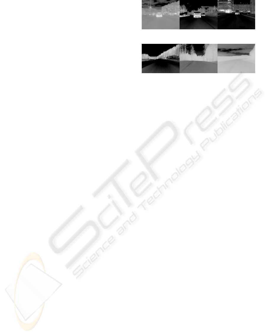
The performance evaluation dataset consists of 8 000
324 × 256 pixel images, half from each category, ex-
tracted from video sequences recorded by a vehicle
mounted infrared sensor. These were gathered dur-
ing night time at various locations in Sweden and
Germany in varying weather conditions. The images
were sampled in the sequences with a constant spatial
interval of 20 meters in city environments and 100
meters in rural environments. Some pre-processing
was carried out to scale the IR intensities to appropri-
ate grey-levels. The ground truth was found by visual
inspection of the video sequences (not individual im-
ages). A few images from the dataset are shown in
Figure 3.
Evaluation was carried out by 4-fold cross vali-
dation on the whole dataset and performed in several
rounds. The primary, exhaustive round was carried
out for GP-Raw, GP-DC and GP-PS to find suitable
values of parameters such as V, n and m. V was var-
ied in the range 16-400, n in the range 5-15 pixels
and m in suitable ranges for each given patch size.
The floating search algorithm is very time consuming,
and was thus not used in this exhaustive evaluation.
Instead vocabularies were generated using k-means
clustering on image elements extracted from 50-300
(a)
(b)
Figure 3: 3 images from the city (a) and rural (b) dataset.
images. Also, classifier parameters were tuned for
optimal performance. Generally, classification per-
formance increases with increasing V and n, and with
decreasing m. It can be seen in Figure 4 that perfor-
mance is good already for vocabularies of sizeV = 16
(for the GP-DC and GP-PS) which is a much smaller
vocabulary size than what has been commonly used
in literature. In fact, vocabularies have shown to be
saturated with information, introducing noisy visual
words already at surprisingly small sizes. The patch
spacing governs the amount of patches extracted from
each image. Small patch spacing gives a larger num-
ber of extracted patches, and thus a more detailed de-
scription, increasing the performance at the cost of
increased time demands. The effect of the patch size
on the classification performance is not as transparent
as the other variables. It affects many different char-
acteristics of the algorithm such as the scale of the
detected objects, the the accuracy of the visual word
matching and the maximum possible complexity of
the visual words. A further discussion is given in
(Forslund, 2008). The GP-PL, GP-CT and GP-HGM
were evaluated separately using suitable parameters.
Though good results were obtained, they were not
surpassing those of the GP-DC and GP-PS methods
when both performance and speed were considered.
Classification results of the different BoW em-
bodiments and the two low-level algorithms are sum-
marised in Table 1. A variety of parameters were
evaluated, but only the best results for each algorithm
are shown in the table. Due to the higher abstrac-
tion level of the BoW model, and the adaptation of
the visual vocabulary to the specific dataset, the BoW
algorithm consistently outperforms the low-level al-
gorithms. Invariant moments are not well suited for
this application since much vital information for the
task lies in the orientation of structures within the
image. The EDH features, which utilise this infor-
mation, perform much better. For varying V Sparse
SIFT consistently performs badly, due to the inability
VISAPP 2010 - International Conference on Computer Vision Theory and Applications
354
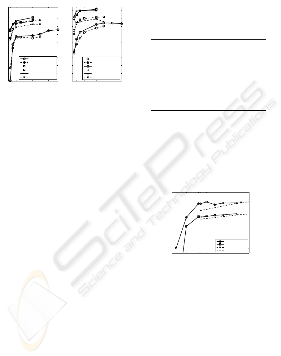
1636 64 100 196 256 324 400
78
80
82
84
86
88
90
92
94
96
Vocabulary Size V
Performance (%)
GP−Raw n = 11, m = 5
GP−Raw n = 5, m = 5
GP−DC n = 11, m = 5
GP−DC n = 5, m = 5
GP−PS n = 11, m = 5
GP−PS n = 5, m = 5
(a)
1636 64 100 196 256 324 400
78
80
82
84
86
88
90
92
94
96
Vocabulary Size V
Performance (%)
GP−Raw n = 11, m = 5
GP−Raw n = 5, m = 5
GP−DC n = 11, m = 5
GP−DC n = 5, m = 5
GP−PS n = 11, m = 5
GP−PS n = 5, m = 5
(b)
Figure 4: The effect of varying the V for a few parameter
variations using (a) SVM and (b) kNN classifier.
of the interest point detector to detect the full con-
tent of the image scene. E.g. large uniform areas,
which are frequent in the rural IR images, are ne-
glected. This is in accordance with the results of
Bosch et al. (Bosch et al., 2008) stating that sparse
extraction is not suitable for scene classification. The
SIFT descriptor, however, is very powerful and ap-
plied densly it demonstrates the best performance of
all methods evaluated in this paper. It is however too
time consuming for the real-time application. Grey
patch based BoW descriptors on the other hand, are
fast to compute and also show good performance. GP-
Raw gives a vocabulary with many redundant visual
words representing homogenous grey-levels; the GP-
DC descriptor was introduced to overcome this issue,
and gives a very good trade off between speed and
performance. The gradient removal approach, GP-
PL, gave interesting vocabularies, but no performance
increase compared to the GP-DC representation. The
histogram based processing GP-HGM and GP-PS,
however, improved the performance compared to GP-
DC for small V (This is not visible in Table 1 since
only the best results of each algorithm are shown).
The histogram based descriptors are however too time
consuming to justify the performance gain and are not
considered for the real-time system.
A suggested real-time vocabulary, denoted RTV
in Table 1, was selected using the GP-DC descrip-
tor to form a vocabulary of size V = 16 using 7 × 7
patches sampled at a spacing of m = 3 pixels. Us-
ing this parameter set, floating search was applied as
described in Section 3.1.2 up to a vocabulary size of
V = 33. Results are displayed, and compared to us-
ing k-means, in Figure 5. For the 16 word vocabulary
used in the RTV, there is a significant performance
gain. To boost the execution speed further, images
were downsampled by a factor s = 2 giving a per-
formance decrease of about 1.5 pp and a four time
Table 1: Summarised results. The best classification perfor-
mance of each algorithm is given in %,(std). Note that pa-
rameters vary between the different algorithms. The RTV is
included for comparison.
Algo. Classif. SVM Classif. kNN
EDH 88.2 (1.7) 90.5 (0.7)
IM 81.0 (0.9) 72.0 (1.7)
GP-Raw 92.8 (1.0) 94.3 (0.9)
GP-DC 96.3 (0.6) 96.7 (0.3)
GP-PL 92.9 (0.7) 96.0 (0.4)
GP-PS 96.3 (0.4) 96.7 (0.4)
GP-HGM 95.4 (0.7) 96.0 (0.4)
S-SIFT 89.1 (1.3) 83.2 (1.5)
D-SIFT 96.3 (0.3) 97.0 (0.4)
RTV 92.7 (0.6) -
speedup. With the SVM parameter ν tuned according
to this configuration to ν = 0.2, and support vectors
stored in single precision, this whole system requires
only 100 kB of memory. The RTV requires about 0.19
s per image (in MATLAB implementation on and In-
tel(R) Core(TM)2 Duo CPU @2.33GHz using 2 GB
of RAM) yielding a maximum allowed frame rate of
about 5.3 Hz, thus within the limits of real-time per-
formance. The classification rate of the RTV is 92.7%
for static images.
4 9 1516 19 23 27 34 36
86
88
90
92
94
96
vocabulary size
performance (%)
Floating search, kNN
Floating search, SVM
K−means, kNN
K−means, SVM
Figure 5: The effect of varyingV for vocabularies generated
using floating search compared to using k-means.
6 CONCLUSIONS
The aim of this paper was to develop a real-time sys-
tem able to separate scenes into the two categories
city and rural scene based on images acquired from
a vehicle mounted IR camera. We used a bag of
words based method utilizing an intermediate seman-
tic representation in the form of a vocabulary of vi-
sual words and compared it to two low-level meth-
ods edge direction histograms and invariant moments.
On a set of images gathered from video sequences,
very high classification performance was obtained for
static scenes when no real-time performance restric-
tions were made (97.0% using BoW with dense SIFT
REAL-TIME ROAD SCENE CLASSIFICATION USING INFRARED IMAGES
355

image element descriptors and V = 400). A proposed
real-time system using BoW with GP-DC image el-
ements and V = 16 gave a performance of 92.7%.
For this, several compromises were made to minimise
time and memory consumption. The choice of GP-
DC as descriptor was made due to speed considera-
tions, but since the problem at hand is of limited com-
plexity, GP-DC showed to provide excellent perfor-
mance, comparable to that of the most complex meth-
ods evaluated. The small vocabulary size was cho-
sen to comply with memory demands, but investiga-
tions showed that the performance converged towards
the maximum for quite small vocabulary sizes (Fig-
ure 4), due to information saturation in the vocabu-
laries. Thus, a very small vocabulary size did not in-
flict serious performance degradations. The quality of
the vocabulary in terms of ability to separate the two
classes was increased notably when floating search
was used to select visual words compared to the com-
monly used k-means clustering. When studying the
misclassified images, many of them (about 30%) were
found to be caused by temporally limited effects such
as passing cars, turns when close to buildings, trees
planted in the city and so on. Thus temporal filtering
of the classification results would increase the general
performance substantially. This is however left as an
issue for further research. Based on this investigation,
we conclude that a road scene classification system
that can be operated during night time at real-time
speed can be constructed to give satisfactory classi-
fication performance.
REFERENCES
Battiato, S., Farinella, G. M., Gallo, G., and Ravì, D.
(2008). Scene categorization using bag of textons on
spatial hierarchy. In ICIP, pages 2536–2539. IEEE.
Bosch, A., Muñoz, X., and Martí, R. (2007). Which is the
best way to organize/classify images by content? Im-
age and Vision Computing, 25(6):778–791.
Bosch, A., Zisserman, A., and Muoz, X. (2008). Scene
classification using a hybrid generative/discriminative
approach. IEEE Transactions on Pattern Analysis and
Machine Intelligence, 30(4):712–727.
Chang, C.-C. and Lin, C.-J. (2001). LIBSVM: a library for
support vector machines. Av. at
http://www.csie.
ntu.edu.tw/~cjlin/libsvm
.
Devendran, V., Thiagarajan, H., and Santra, A. K. (2007).
Scene categorization using invariant moments and
neural networks. In Proceedings of ICCIMA, vol-
ume 1, pages 164–168.
Forslund, D. (2008). Realtime scene analysis in infrared
images. Master’s thesis, Uppsala University, Sweden.
Hu, M.-K. (1962). Visual pattern recognition by moment
invariants. IRE Transactions on Information Theory,
8(2):179–187.
Lowe, D. (2004). Distinctive image features from scale-
invariant keypoints. Int. Journal of Computer Vision,
60(2):91–110.
Oliva, A. and Torralba, A. (2001). Modeling the shape of
the scene: A holistic representation of the spatial en-
velope. Int. Journal of Computer Vision, 42(3):145–
175.
Oliva, A. and Torralba, A. (2003). Statistics of natural im-
age categories. Network: Computation in Neural Sys-
tems, pages 391–412.
Pudil, P., Ferri, F., Novovicova, J., and Kittler, J. (1994).
Floating search methods for feature selection with
nonmonotonic criterion functions. In ICPR94, pages
279–283.
Quelhas, P., Monay, F., Odobez, J. M., Gatica-Perez, D.,
Tuytelaars, T., and Van Gool, L. (2005). Modeling
scenes with local descriptors and latent aspects. In
Tenth IEEE Int. Conf. on Computer Vision, 2005, vol-
ume 1, pages 883–890.
Sivic, J. and Zisserman, A. (2003). Video google: a text re-
trieval approach to object matching in videos. In Ninth
IEEE Int. Conf. on Computer Vision, 2003, pages
1470–1477.
Szummer, M. and Picard, R. W. (1998). Indoor-outdoor
image classification. In Proceedings of the 1998
Int. Workshop on Content-Based Access of Image and
Video Databases, page 42.
Vailaya, A., Figueiredo, M. A. T., Jain, A. K., and Zhang,
H.-J. (2001). Image classification for content-based
indexing. IEEE Transactions on Image Processing,
10(1):117–130.
Vailaya, A., Jain, A., and Zhang, H. J. (1998). On image
classification: City vs. landscape. In Proceedings of
the IEEE Workshop on Content - Based Access of Im-
age and Video Libraries, pages 3–8.
Walker, L. L. and Malik, J. (2003). When is scene
recognition just texture recognition. Vision Research,
44:2301–2311.
VISAPP 2010 - International Conference on Computer Vision Theory and Applications
356
